Large-scale multi-agent transportation simulations

Dept. of Computer Science, ETH Zürich, Switzerland
Postal: ETH Zentrum IFW B27.1, CH-8092 Zürich, Switzerland
Phone: +41 1 632 5427, Fax: +41 1 632 1374

Abstract:

It is now possible to microsimulate the traffic of whole metropolitan areas with 10 million travelers or more, ``micro'' meaning that each traveler is resolved individually as a particle. In contrast to physics or chemistry, these particles have internal intelligence; for example, they know where they are going. This means that a transportation simulation project will have, besides the traffic microsimulation, modules which model this intelligent behavior. The most important modules are for route generation and for demand generation. Demand is generated by each individual in the simulation making a plan of activities such as sleeping, eating, working, shopping, etc. If activities are planned at different locations, they obviously generate demand for transportation. This however is not enough since those plans are influenced by congestion which initially is not known. This is solved via a relaxation method, which means iterating back and forth between the activities/routes generation and the traffic simulation.

$\begin{keyword} traffic simulation, transportation planning, queue model, TRANSIMS, parallel computing \PACS{07.05.Tp, 89.40.+k, 89.50.+r} \end{keyword}$

Introduction

Cars finding their way through a street network resemble, say, electrons finding their way through a resistor network. This means that one can use microscopic simulation methods, such as cellular automata or molecular dynamics simulations. In order to be as realistic as possible, one might think that different kinds of drivers are needed, such as people with poor or educated driving skills or people driving aggressively or in a calm manner. But it turns out that, similar to physics, in many cases this is not necessary; it is sufficient to introduce some randomness into every time step (annealed vs. quenched randomness).

There is however a fundamental difference between cars and electrons: Cars typically have a destination, which makes the particles distinguishable, and any mathematical approach considerably more difficult. In consequence, much progress in recent years was based on the use of computers. These simulation models indeed resemble cellular automata or molecular dynamics, or sometimes smooth particle hydrodynamics simulations. The particles (vehicles) however carry considerably more intelligence, for example about their route and their final destination.

TRANSIMS

The TRANSIMS (TRansportation ANalysis and SIMulation System) [1] is a microsimulation project for transportation planning developed at Los Alamos National Laboratory. Transportation planning is typically done for large regional areas with several millions of travelers, and it is done with 20-year time horizons. This has two meanings: First, a microsimulation approach needs to simulate large enough areas fast enough. Second, the methodology needs to be able to pick up aspects like induced travel, where people change their activities and maybe their home locations because of changed impedances of the transportation system. Based on these issues, TRANSIMS consists of the following modules (Fig. 1):

This means that the microsimulation needs to be run more than once - in our experience about fifty times for a relaxation from scratch [7,8]. In consequence, a computing time that may be acceptable for a single run is no longer acceptable for such a relaxation series - thus putting an even higher demand on the technology.

**Figure 1:** TRANSIMS design
$\includegraphics[width=\hsize]{transims-bubbles-fig.eps}$

Cellular automata and queue model simulation of traffic

Human behavior can be complex. It is a challenge throughout projects such as this one to simplify the rules of behavior for the computer implementation and still obtain useful results. There is for example a considerable amount of work about cellular automata models for car traffic [9], which is also the method used by TRANSIMS [10].

Defining ``useful results'' depends on the question. For TRANSIMS which is designed for transportation planning, many important aspects depend on link travel times. These in turn depend on delays caused by congestion, and congestion is caused by demand being higher than capacity. Thus, the problem to be solved is how to handle the capacity constraints of the road network, such as maximum flow on freeways, traffic lights on arterials and opposing traffic flows in case of unprotected turns. The CA approach generates the correct behavior from a few basic parameters such as noise parameter in the acceleration on freeways and on arterials or gap acceptance for unprotected turns. An even simpler alternative is a queue model [11,12]. Basically, within this model, each link is represented by a queue with a free flow velocity $v_{0}$ , a length $L$ , a flow capacity $C$ and a number of lanes $n_{lanes}$ ; these values are given by the input files. Free flow velocity is the velocity of traffic when the traffic density is very low. Free flow travel time is given by the relation $T_{0} = {L / v_{0}}$ .

We have two different capacity constraints related to each link. The flow capacity limits the number of vehicles that are allowed to leave the link. The storage capacity, on the other hand, controls the number of the vehicles that are allowed to enter the link. If one assumes that the space a vehicle occupies in congestion is $l_{veh} = 7.5$ m, then the maximum number of vehicles that a link can contain is $N_{sites} = {L \cdot n_{lanes}}/ l_{veh}$ . This is the storage capacity.

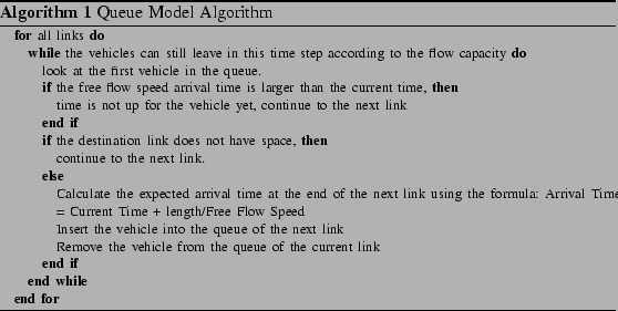
Vehicles then move according to their plans in this queue simulation. When they enter a link, they are added at the end of a queue. When all vehicles in front of them have left, then it is their turn to leave the link. The dynamics for the queue model is implemented using the algorithm shown in Algorithm 1. This is very similar to a queuing simulation except that the links have the storage capacity constraint.

$\begin{algorithm} % latex2html id marker 87\caption{Queue Model Algorithm} \s... ... current link} \ENDIF \ENDWHILE \ENDFOR \end{algorithmic}\end{algorithm}$

Relaxation of plans via iteration

As said above, we perform iterations between the traffic microsimulator and the route planner. The microsimulator, whether queue-based or TRANSIMS, models individual drivers as they interact on the roadways of the traffic network. The route planner pre-plans each driver's route before the microsimulation runs.

The route planner simply finds the fastest path for each driver, from pre-determined starting and destination points, based on the known average travel times (based on traffic flow aggregated over 15-minute intervals) of vehicles on each link in the network. Only at the beginning of the iteration series, this information does not exist, since no vehicles have been simulated yet. So, the router initially uses the free-flow speeds of the links to obtain ``naive'' travel times of the links for an empty network. In effect, each driver plans his or her route as if he or she will never encounter another vehicle on the road. This means vehicles are likely to use the same roads (the ones with the higher free speeds), and cause extreme traffic on those links, while leaving other links almost completely free of traffic.

Once the microsimulation has run for the first time, we take the travel times experienced by vehicles on the links for each 15-minute time interval and feed them back into the router, which generates another set of plans. The router does not re-plan all the drivers, because this would cause them all to switch to the same new alternatives while ignoring the roads previously congested. Instead, it chooses 10% of the drivers at random, and gives them new plans based on the new data. The complete set of plans (90% old, 10% new) is given to the microsimulator again, and the cycle is repeated until the plans ``relax'' to a realistic scenario, where nobody can gain any advantage by choosing a new plan.

Gotthard Scenario

We use the so-called Gotthard Scenario to test our simulations for plausibility. In this scenario, we simulate the traffic resulting from 50,000 vehicles which start between 6 a.m. and 7 a.m. all over Switzerland and which all want to travel to Lugano, which is in the Ticino, the Italian-speaking part of Switzerland south of the Alps. In order for the vehicles to get there, most of them have to cross the Alps. There are however not many ways to do this, resulting in traffic jams, most notably at the Gotthard tunnel. This scenario has some resemblance with real-world vacation traffic in Switzerland.

Fig. 2 shows a typical result. We compare the 15-minute aggregated density of the links in the simulated road network, which is calculated for a given link by dividing the number of vehicles seen on that link in a 15-minute time interval by the length of the link (in meters) and the number of traffic lanes the link contains. In all of the figures, the network is drawn as the set of small, connected line segments, re-creating the roadways as might be seen from an aerial or satellite view of the country. The lane-wise density values are plotted for each link as a 3-dimensional box super-imposed on the 2-dimensional network, with the base of a box lying on top of its corresponding link in the network, and the height above the ``ground'' set relative to the value of the density. Thus, larger density values are drawn as taller boxes, and smaller values with shorter boxes. (The ``camera'' angle of the figures was chosen to emphasize the height of the boxes in the southern region of Switzerland, where all the ``interesting'' data comes from. This causes the ``up'' direction to be slanted to the left.) Longer links naturally have longer boxes than shorter links. Also, the boxes are color-coded, with smaller values tending towards green, middle values tending towards yellow, and larger values tending towards red. In short, the higher the density (the taller/redder the boxes), the more vehicles there were on the link during the 15-minute time period being illustrated. Higher densities imply higher vehicular flow, up to a certain point (probably the yellow boxes), but any boxes that are orange or red generally indicate a congested (jammed) link. All times given in the figures are at the end of a 15-minute measurement interval. Thus, figure 2 illustrates the density calculated from vehicle counts taken between 7:45 and 8:00 a.m.

Qualitatively, the overall results of both simulations are similar. Congestion occurs in the expected places in both simulations. The TRANSIMS simulation moves vehicles more slowly in general, as is evidenced by the TRANSIMS simulation jams lagging behind their Queue simulation counterparts, and the fact that the TRANSIMS simulation requires more simulated time to allow all of its vehicles to arrive at their destination.

**Figure 2:** Snapshots at 8:00 a.m. *Top:*From TRANSIMS, *Bottom:*From Queue Model.
[width=]transims/8amLFlow.ps [width=]queue/8amLFlow.ps

Fig. 3 gives similar information in a different format. Plotted is, for each link of the network, the flow between 7 a.m. and 8 a.m. of the TRANSIMS simulation on the x-axis vs. the flow of the Queue simulation on the y-axis. Again, it is clear that the results are strongly correlated, but there are also large differences.

At this point, it seems hard to go beyond these general remarks without field data to compare with. Our next step will be the simulation of traffic on a normal workday in Switzerland. For these results, it will then be possible to make comparisons to field data, which will allow further conclusions regarding the validity of our results and further improvements. For such results for a scenario in Portland/Oregon, see [13].

**Figure 3:** Link-by-link comparison of flows from 7 a.m. to 8 a.m. between TRANSIMS and the Queue simulation for the Gotthard Scenario.
$\includegraphics[width=\hsize]{scatter-gpl.eps}$

Computational issues

As mentioned above, computational speed is an important aspect of this work. A metropolitan region can consist of 10 million or more inhabitants; and in contrast to molecular dynamics (MD) simulations, traffic ``particles'' (

travelers, vehicles) have considerably more internal intelligence than MD particles. This internal intelligence translates into rule-based code, which does not vectorize but runs well on modern workstation architectures. This makes traffic simulations ideally suited for clusters of PCs, also called Beowulf clusters. We use domain decomposition, that is, each CPU obtains a patch of the geographical region. Information and vehicles between the patches are exchanged via message passing using MPI (Message Passing Interface).

Fig. 4 shows computing speed predictions for TRANSIMS as a function of the number of CPUs. The real time ratio (RTR) is the factor the simulation runs faster than reality; and RTR of 10 means for example that 10 hours of traffic can be simulated during 1 hour of computer time. The curves refer to a network of the city of Portland (Oregon) with 20,000 links (i.e. a number of links similar to our Switzerland network, but all of them much shorter).

As indicated in the figure, the different lines refer to different computing architectures. The thick line refers to a Beowulf cluster consisting of 500 MHz Pentium CPUs connected via standard 100 Mbit switched Ethernet. The black dots show actual computational speed measurements on the same architecture. One clearly sees that up to about 32 CPUs the Beowulf architecture is fairly efficient for this problem size and computing speeds more than 50 times faster than real time can be reached. One also sees the typical ``leveling out'' of the curve for higher numbers of CPUs. The impediment to higher computational speed here is the latency of Ethernet, in contrast to many other simulations, where it is the bandwidth.

The ``short-dashed'' line shows what would happen if one dispensed with the switch in the Ethernet. In fact, for large numbers of CPUs the Ethernet switch becomes a major part of the cost of such a cluster - alternatively one uses a switch without enough bandwidth which would result in a curve between the red and the blue.

The ``long-dashed'' line refers to running the same problem on the ASCI Blue Mountain supercomputer which is essentially a cluster of 200 MHz SGI Origin computing nodes coupled via a high-performance low-latency communication network. Due to the smaller CPU speed, the curve starts at a lower position, and only with more than 64 CPUs the use of the much more expensive supercomputer pays off.

Finally, the dotted line refers to a problem size ten times larger running again on a Pentium cluster with 100 Mbit switched Ethernet. This problem size corresponds approximately to our simulations of all of Switzerland. Here one sees the typical ``scale-up'' phenomenon of parallel computing, where one can increase the problem size without decrease of computational speed as long as one can add CPUs accordingly.

The computational speed predictions are done by adding up the times incurred by computing, latency, node bandwidth restrictions, and network bandwidth restrictions. For more information, see [14].

**Figure 4:** Computational speed for TRANSIMS. The ``dip'' in the measured values at 24 CPUs is due to the fact that 24 CPUs are connected to a single Ethernet switch, which in turn is connected to another switch to gain access to further CPUs.
[width=]rtr-gpl.eps

Summary

Large-scale microscopic traffic simulation packages for transportation planning consist of at least four modules: synthetic population generation, activities generation (demand generation), route planner, and the traffic microsimulation itself. These modules need to be consistent; for example, expectations about congestion in the route planner need to be consistent with actually encountered congestion in the traffic microsimulation. This is achieved by using a relaxation method.

Due to the large problem size (

``particles'' times

time steps times

iterations), the computing demands are high. The use of Beowulf parallel computers is an effective yet affordable way to handle these demands.

Bibliography

About this document ...

This document was generated using the LaTeX2HTML translator Version 2K.1beta (1.47)

The command line arguments were:
latex2html -split 1 -dir html aachen01_CmpPhys.tex