Status of a TRANSIMS implementation for Switzerland

Andreas Voellmy${}^a$, Milenko Vrtic${}^b$, Bryan Raney${}^a$,
Kay Axhausen${}^b$, and Kai Nagel${}^a$
${}^a$ Dept. of Computer Science, ETH Zürich
CH-8092 Zürich, Switzerland
${}^b$ Dept. of Civil Engineering, IVT, ETH Zürich
CH-8093 Zürich, Switzerland

Abstract:

TRANSIMS (TRansportation ANalysis and SIMulation System) is a microscopic simulation package for transportation planning, ``microscopic'' meaning that each traveler is resolved individually as a particle. This package is used with the goal of simulating 24-hours of all the traffic in Switzerland. This is used to ``stress-test'' TRANSIMS with respect to its capability to simulate large metropolitan areas with 10 million travelers or more. This paper gives an overview of the current status.

Introduction

The TRANSIMS (TRansportation ANalysis and SIMulation System) project at the Los Alamos National Laboratory is a multi-year, multi-million dollar project to write a microscopic simulation package for transportation planning. Microscopic means that all objects of the simulation, such as travelers but also roads, intersections, traffic lights, etc., are resolved individually. TRANSIMS is designed for large metropolitan areas with several million travelers, such as New York or Los Angeles.

In order to stress-test TRANSIMS, we are in the process of implementing a 24-hour simulation of TRANSIMS for the whole country of Switzerland. Switzerland has 7.2 million inhabitants; including transit traffic, traffic into or out of Switzerland, and freight traffic this will result in about 20-25 million trips. The goal of this study is twofold:

• Investigate if it is possible to make TRANSIMS realistic enough to be useful for such a scenario, and how difficult this is.

• Investigate the computational challenges and how they can be overcome.

This paper gives a short report on the current status. Sec. 2 describes the TRANSIMS modules. Sec. 3 then describes the input data and how they were adapted for the purposes of this study. In particular, besides the normal demand we also describe one that we have designed for testing purposes, and where 50000 travelers travel from random starting points within Switzerland to the Ticino, which is the southern part of Switzerland. We use this second scenario as a plausibility test for routing and feedback. This is followed by Sec. 4, which describes some results.

TRANSIMS modules

Figure 1: TRANSIMS design

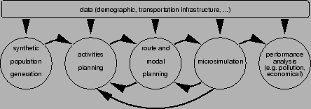
TRANSIMS consists of the following modules (Fig. 1):

• Population generation. Demographic data is disaggregated so that one obtains individual households and individual household members, with certain characteristics, such as a street address, car ownership, or household income [1]. - This module is not used for our current investigations but will be used in the future.

• Activities generation. For each individual, a set of activities (home, going shopping, going to work, etc.) and activity locations for a day is generated [2,3]. - This module is not used in our current investigations but will be used in the future.

• Modal and route choice. For each individual, modes and routes are generated that connect activities at different locations [4].

• Traffic micro-simulation. Up to here, all individuals have made plans about their behavior. The traffic micro-simulation executes all those plans simultaneously [5]. In particular, we now obtain the result of interactions between the plans - for example congestion.

• Feedback. In addition, such an approach needs to make the modules consistent with each other. For example, plans depend on congestion, but congestion depends on plans. A widely accepted method to resolve this is systematic relaxation (e.g. [6]) - that is, make preliminary plans, run the traffic micro-simulation, adjust the plans, run the traffic micro-simulation again, etc., until consistency between modules is reached. The method is somewhat similar to the Frank-Wolfe-algorithm in static assignment (see, e.g., Ref. [7], ``convex combinations method''), or in more general terms to a standard relaxation technique in numerical analysis.

Since this approach is modular, TRANSIMS modules can be replace by other modules. This can be of advantage, e.g., for research reasons, or in order to adapt to local circumstances. In our current work, the population generation and the activities generation are replaced by a more conventional approach based on origin-destination-matrices. This is described in Secs. 3.2 and  3.3. The remaining modules are the router, the traffic micro-simulation, and the feedback. They will be described in more detail in the following.

Routing

TRANSIMS in general has the provision for arbitrary modes of transportation. Even if a mode is not implemented in the micro-simulation (see below), it is still possible to generate a route for it and thus obtain an estimate for the resulting travel time and inconvenience. Currently, we do however assume that all travel is done by using cars. This will lead to an over-estimation of car traffic in realistic scenarios.

The router is adaptive to congestion. It uses a time-dependent Dijkstra algorithm. Link travel times are fed back from the micro-simulation in 15-min time bins, and the router finds the fastest route based on these 15-min time bins. It is assumed that ``waiting at nodes'' can never lead to improvements - this is justified since in reality links behave approximately as FIFO (first-in first-out) queues. Apart from that, the implementation of a time-dependent Dijkstra algorithm is standard [4].

Micro-simulation

The TRANSIMS micro-simulation is a complex package with many rules and details. In order to speed up the computation, the underlying driving rules are based on the cellular automaton (CA) method [8] with additional rules for lane changing and protected as well as unprotected turns. A detailed description of these rules can be found in Ref. [5]. The result is, within the limits of the capabilities of a CA, a virtual reality traffic simulation. Note that besides the usual traffic dynamics, vehicles also follow routes as specified above. This means, for example, that vehicles need to change lanes in order to be in one of the allowed lanes for the desired turning movement. Vehicles which fail to do this because of too much traffic are removed from the simulation.

Feedback

As mentioned above, plans (such as routes) and congestion need to be made consistent. This is achieved via a relaxation technique:

1. Initially, the system generates a set of routes based on free speed travel times.

2. The traffic simulation is run with these routes.

3. 10% of the population obtains new routes, which are based on the link travel times of the last traffic simulation.

4. This cycle is run for 50 times; earlier investigations have shown that this is more than enough to reach relaxation [9].

Note again that this implies that routes are fixed during the traffic simulation and can only be changed between micro-simulation runs (``between-day replanning''). Work is under way to improve this situation, i.e. to allow within-day replanning.

Input data and scenarios

The Switzerland network

The network used was orignally developed for the Swiss regional planning authority (Bundesamt für Raumentwicklung). It has since been updated, corrected and calibrated by one of us (Vrtic). The 3066 zones contained within the network correspond to the local authorities (Gemeinden) and in the larger cities to the various official within-authority subdivisions (Stadtkreise). These zones are sometimes called Traffic Analysis Zones (TAZs). The network has the fairly typical number of 10572 nodes and 28622 links. Also fairly typical, the major attributes on these links are type, length, speed, and capacity. Since the TRANSIMS micro-simulation is extremely realistic with respect to details such as number of lanes, turn and merge lanes, lane connectivity across intersections, or traffic signal phases, plausible defaults need to be generated for those elements from the available network files. Some of the heuristics used during this process are the following:

• The number of lanes is uniformly set to one per direction except for freeways inside Switzerland where the correct number of lanes is used.

• All intersections are assumed as ``no control'', which is a TRANSIMS category meaning that the simulation does not make any special provisions in order to deal with traffic stream priorities. The result will depend on the sequence in which the simulation goes through the links. - This is a major shortcoming of our current status; work to correct it is under way but will take time.

• TRANSIMS needs lane connectivity across intersections in order to function properly. For 1-lane links, all incoming links are connected to all outgoing links. For multilane links, the lanes are essentially connected ``in parallel;'' that is, lane 1 on the incoming link to lane 1 on the outgoing link, lane 2 on the incoming link to lane 2 on the outgoing link, etc. On- and off-ramps are connected to the shoulder lane. Special care is taken at the beginning and ending of multilane roads: If $n$ incoming single-lane roads are connected to an outgoing $n$-lane road, then each incoming link obtains its own outgoing lane. - There are however cases which are not covered adequately by our approach. Problematic layouts are corrected on a case-by-case basis; work for a more systematic approach is under way but will take time.

Demand generation for the Gotthard scenario

In order to test our set-up, we generated a set of 50000 trips all going to the same destination. All trips going to the same destination allows us to check the plausibility of the feedback since all traffic jams on all used routes to the destination should dissolve in parallel. In this scenario, we simulate the traffic resulting from 50000 vehicles which start between 6am and 7am all over Switzerland and which all go to Lugano, which is in the Ticino, the Italian-speaking part of Switzerland south of the Alps. In order for the vehicles to get there, most of them have to cross the Alps. There are however not many ways to do this, resulting in traffic jams, most notably in the corridor leading towards the Gotthard pass. This scenario has some resemblance with real-world vacation traffic in Switzerland.

Demand generation for the Switzerland scenario

Our starting point for demand generation for the full Switzerland scenario are 24-hour origin-destination matrices from the Swiss regional planning authority (Bundesamt für Raumentwicklung). Eventually, we intend to move on to activity-based demand generation.

The original 24-hour matrix is converted into 24 one-hour matrixes using a three step heuristic. The first step employs departure time probabilities by population size of origin zone, population size of destination zone and network distance. These are calculated using the 1994 Swiss National Travel Survey (Mikrozensus 1994). The resulting 24 initial matrices are then corrected (calibrated) using the OD-matrix estimation module of one of the macroscopic assignment environments used at the IVT (VISUM; PTV AG, 2001). Hourly counts are available from the counting stations on the national motorway system. Finally, the hourly matrices are rescaled so that the totals over 24 hours matched the original 24h matrix.

A dynamic macroscopic assignment of the matrices shows that the patterns of congestion over time are realistic and consistent with the known patterns. A more detailed verification was not possible so far, but is planned for 2002.

These hourly matrices are then disaggretated into individual trips. That is, we generate individual trips such that summing up the trips would again result in the given OD matrix. The starting time for each trip is randomly selected between the starting and the ending time of the validity of the OD matrix.

The OD matrices assume traffic analysis zones (TAZs) while in TRANSIMS the assumption is that traffic starts on so-called parking accessories which are proxies for parking spaces along each individual link. We use one parking accessory for each link. We convert traffic analysis zones to Parking Accessories by the following heuristic:

• The geographic location of the zone is found via the geographical coordinate of its centroid given by the data base.

• A circle with radius 3 km is drawn around the centroid.

• Each link starting within this circle is now a possible starting link for the trips. One of these links is randomly selected and the trip start or end is assigned.

This leads to a list of approximately 11 million trips. Since the origin-destination matrices are given on an hourly basis, these trips reflect the daily dynamics. Note that inter-zonal trips are not included in those matrices, as by tradition.

Some results

Fig. 2 shows a typical result for the Gotthard scenario. The figures show the 15-minute aggregated density of the links in the simulated road network, which is calculated for a given link by dividing the number of vehicles seen on that link in a 15-minute time interval by the length of the link (in meters) and the number of traffic lanes the lane contains. In all of the figures, the network is drawn as the set of small, connected line segments, re-creating the roadways as might be seen from an aerial or satellite view of the country. The lane-wise density values are plotted for each link as a 3-dimensional box super-imposed on the 2-dimensional network, with the base of a box lying on top of its corresponding link in the network, and the height above the ``ground'' set relative to the value of the density. Thus, larger density values are drawn as taller boxes, and smaller values with shorter boxes. (The ``camera'' angle of the figures was chosen to emphasize the height of the boxes in southern region of Switzerland, where all the ``interesting'' data comes from. This causes the ``up'' direction to be slanted to the left.) Longer links naturally have longer boxes than shorter links. Also, the boxes are color coded, with smaller values tending toward green, middle values tending toward yellow, and larger values tending toward red. In short, the higher the density (the taller/redder the boxes), the more vehicles there were on the link during the 15-minute time period being illustrated. Higher densities imply higher vehicular flow, up to a certain point (the yellow boxes), but any boxes that are orange or red indicate a congested (jammed) link. All times given in the figures are at the end of the 15-minute measurement interval. The Gotthard tunnel and the destination in Lugano are indicated in the top picture; Lugano is also seen in the middle of the red cluster near the bottom of the bottom figure.

As expected, many routes towards the single destination are equally used. In particular, many longer but uncongested routes are used in the final iteration (shown here) which are initially empty. It turns however out that only a subset of routes towards the final destination is used. This is related to the unrealistic intersection dynamics caused by the ``no control'' intersections: There are many plausible routes which are at a disadvantage at critical intersections and which are for that reason used by very few vehicles.

Fig. 3 shows a preliminary result of the Switzerland scenario. In particular, this is a result before any feedback iterations were done. As one would expect, there is more traffic near the cities than in the country.

Figure 2: Snapshots at 8:00AM and 11:00AM. The circle shows the traffic jam before the Gotthard tunnel. The arrow indicates the destination of all vehicles.

[width=0.8]8am-gz.eps

[width=0.8]11am-tif.eps

Figure 3: Switzerland at 8AM. Very preliminary result. The plot shows our network of Switzerland, plus each vehicle in the network as a pixel. Vehicles with low speed are in black, vehicles which travel at free speed are in light gray. In consequence, congested areas are shown in black.

Computational issues

Figure 4: Computational speed for a Beowulf cluster with 500 MHz CPUs and 100 Mbit Ethernet. The black dots are measurements; the line is a model-based prediction based on the same measurements. The model assumes a full-bandwidth Ethernet switch, which becomes a major cost factor with larger numbers of CPUs.

[width=0.8]rtr-gpl.eps

A metropolitan region can consist of 10 million or more inhabitants, the simulation of whom causes considerable demands on computational performance. This demand is made worse by the repeated execution of the relaxation iterations. And in contrast to simulations in the natural sciences, traffic particles (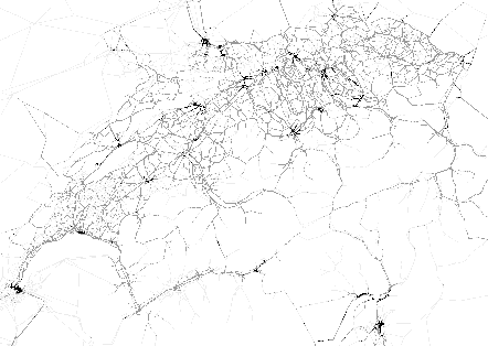$=$ travelers, vehicles) have internal intelligence. This internal intelligence translates into rule-based code, which does not vectorize. It however runs well on modern workstation architectures, which makes traffic simulations ideally suited for clusters of PCs, also called Beowulf clusters. We use domain decomposition, that is, each CPU obtains a patch of the geographical region. Information and vehicles are exchanged between the patches via message passing using MPI (Message Passing Interface).

Fig. 4 shows measured and predicted computing speeds as a function of the number of CPUs. The prediction is based on a theoretical model of computational performance whose parameters are found using the performance measurements [10]. The real time ratio (RTR) is the factor which compares the simulation speed to reality; an RTR of 10, for example, means that 10 hours of traffic can be simulated during 1 hour of computer time. The curves refer to a network of the city of Portland (Oregon) with 20000 links (i.e. a similar number of links as our Switzerland network, but all of them much shorter).

One clearly sees that up to about 32 CPUs the Beowulf architecture is fairly efficient for this problem size and computing speeds of more than 50 times faster than real time can be reached. One also sees the typical ``leveling out'' of the curve for higher numbers of CPUs. The impediment to higher computational speed is the latency of Ethernet, in contrast to many other simulations, where it is the bandwidth. For more information and predictions for other architectures, see [10].

Summary

In terms of travelers and trips, a simulation of all of Switzerland is comparable with a simululation of a large metropolitan area, such as London or Los Angeles. This is used as a test-bed to ``stress-test'' TRANSIMS, in particular the TRANSIMS micro-simulation. The goal is a full 24-hour simulation of all traffic within Switzerland. The starting point is a conversion of the Swiss transportation planning network into a network which can be used by TRANSIMS. This includes the generation of default layouts for intersections etc. Demand is generated from converted 24-hour origin-destination matrices, but will in future come from activities. A second demand set was generated for testing purposes. Routes are computed as time-dependent fastest path; additional modes besides cars will be included in the future. The simulation runs on a network of coupled Pentium computers. Although considerable progress has been made, much work remains still to be done.

Bibliography

1

R. J. Beckman, K. A. Baggerly, and M. D. McKay.
Creating synthetic base-line populations.
Transportion Research Part A - Policy and Practice, 30(6):415-429, 1996.

2

K.M. Vaughn, P. Speckman, and E.I. Pas.
Generating household activity-travel patterns (HATPs) for synthetic populations, 1997.

3

J. L. Bowman.
The day activity schedule approach to travel demand analysis.
PhD thesis, Massachusetts Institute of Technology, Boston, MA, 1998.

4

R. R. Jacob, M. V. Marathe, and K. Nagel.
A computational study of routing algorithms for realistic transportation networks.
ACM Journal of Experimental Algorithms, 4(1999es, Article No. 6), 1999.

5

K. Nagel, P. Stretz, M. Pieck, S. Leckey, R. Donnelly, and C. L. Barrett.
TRANSIMS traffic flow characteristics.
Los Alamos Unclassified Report (LA-UR) 97-3530, 1997.

6

J. A. Bottom.
Consistent anticipatory route guidance.
PhD thesis, Massachusetts Institute of Technology, Cambridge, MA, 2000.

7

Y. Sheffi.
Urban transportation networks: Equilibrium analysis with mathematical programming methods.
Prentice-Hall, Englewood Cliffs, NJ, USA, 1985.

8

K. Nagel and M. Schreckenberg.
A cellular automaton model for freeway traffic.
Journal de Physique I France, 2:2221, 1992.

9

M. Rickert.
Traffic simulation on distributed memory computers.
PhD thesis, University of Cologne, Germany, 1998.
See www.zpr.uni-koeln.de/~mr/dissertation.

10

K. Nagel and M. Rickert.
Parallel implementation of the TRANSIMS micro-simulation.
Parallel Computing, 27(12):1611-1639, 2001.

About this document ...

Status of a TRANSIMS implementation for Switzerland

This document was generated using the LaTeX2HTML translator Version 2K.1beta (1.47)

Copyright © 1993, 1994, 1995, 1996, Nikos Drakos, Computer Based Learning Unit, University of Leeds.
Copyright © 1997, 1998, 1999, Ross Moore, Mathematics Department, Macquarie University, Sydney.

The command line arguments were:
latex2html -split 1 -dir html nets-sp-issue.tex

The translation was initiated by Kai Nagel on 2001-12-12