![]()
![]()
and Marcus Rickertmr
sd&m AG, Troisdorf, Germany
Apart from typographical and layout changes, this version should :-) be identical to the printed version.
We then demonstrate how computing speeds of our parallel micro-simulations can be systematically predicted once the scenario and the computer architecture are known. This makes it possible, for example, to decide if a certain study is feasible with a certain computing budget, and how to invest that budget. The main ingredients of the prediction are knowledge about the parallel implementation of the micro-simulation, knowledge about the characteristics of the partitioning of the transportation network graph, and knowledge about the interaction of these quantities with the computer system. In particular, we investigate the differences between switched and non-switched topologies, and the effects of 10 Mbit, 100 Mbit, and Gbit Ethernet.
As one example, we show that with a common technology - 100 Mbit switched Ethernet - one can run the 20000-link EMME/2-network for Portland (Oregon) more than 20 times faster than real time on 16 coupled Pentium CPUs.

It is by now widely accepted that it is worth investigating if the microscopic simulation of large transportation systems [7,42] is a useful addition to the existing set of tools. By ``microscopic'' we mean that all entities of the system - travelers, vehicles, traffic lights, intersections, etc. - are represented as individual objects in the simulation [15,33,16,32,13,21,44].
The conceptual advantage of a micro-simulation is that in principle it can be made arbitrarily realistic. Indeed, microscopic simulations have been used for many decades for problems of relatively small scale, such as intersection design or signal phasing. What is new is that it is now possible to use microscopic simulations also for really large systems, such as whole regions with several millions of travelers. At the heart of this are several converging developments:
In consequence, for situations where one expects that the fluid-dynamical representation of traffic is realistic enough for the dynamics but one wants access to individual vehicles/drivers/..., a simple microscopic simulation may be the solution. In addition to this, with the microscopic approach it is always possible to make it more realistic at some later point. This is much harder and sometimes impossible with macroscopic models.
The TRANSIMS (TRansportation ANalysis and SIMulation System) project at Los Alamos National Laboratory [42] is such a micro-simulation project, with the goal to use micro-simulation for transportation planning. Transportation planning is typically done for large regional areas with several millions of travelers, and it is done with 20 year time horizons. The first means that, if we want to do a micro-simulation approach, we need to be able to simulate large enough areas fast enough. The second means that the methodology needs to be able to pick up aspects like induced travel, where people change their activities and maybe their home locations because of changed impedances of the transportation system. As an answer, TRANSIMS consists of the following modules:
The reason why this is important in the context of this paper is that it means that the micro-simulation needs to be run more than once - in our experience about fifty times for a relaxation from scratch [34,35]. In consequence, a computing time that may be acceptable for a single run is no longer acceptable for such a relaxation series - thus putting an even higher demand on the technology.
This can be made more concrete by the following arguments:
This paper will concentrate on the microsimulation of TRANSIMS. The other modules are important, but they are less critical for computing (see also Sec. 10). We start with a description of the most important aspects of the TRANSIMS driving logic (Sec. 3). The driving logic is designed in a way that it allows domain decomposition as a parallelization strategy, which is explained in Sec. 4. We then demonstrate that the implemented driving logic generates realistic macroscopic traffic flow. Once one knows that the microsimulation can be partitioned, the question becomes how to partition the street network graph. This is described in Sec. 6. Sec. 7 discusses how we adapt the graph partitioning to the different computational loads caused by different traffic on different streets. These and additional arguments are then used to develop a methodology for the prediction of computing speeds (Sec. 8). This is rather important, since with this one can predict if certain investments in one's computer system will make it possible to run certain problems or not. We then shortly discuss what all this means for complete studies (Sec. 10). This is followed by a summary.
As mentioned above, micro-simulation of traffic, that is, the individual simulation of each vehicle, has been done for quite some time (e.g. [17]). A prominent example is NETSIM [15,33], which was developed in the 70s. Newer models are, e.g., the Wiedemann-model [45], AIMSUN [16], INTEGRATION [32], MITSIM [13], HUTSIM [21], or VISSIM [44].
NETSIM was even tried on a vector supercomputer [23], without a real break-through in computing speeds. But, as pointed out earlier, ultimately the inherent structure of agent-based micro-simulation is at odds with the computer architecture of vector supercomputers, and so not much progress was made on the supercomputing end of micro-simulations until the parallel supercomputers became available. One should note that the programming model behind so-called Single Instruction Multiple Data (SIMD) parallel computers is very similar to the one of vector supercomputers and thus also problematic for agent-based simulations. In this paper, when we talk about parallel computers, we mean in all cases Multiple Instruction Multiple Data (MIMD) machines.
Early use of parallel computing in the transportation community includes parallelization of fluid-dynamical models for traffic [10] and parallelization of assignment models [18]. Early implementations of parallel micro-simulations can be found in [9,29,1].
It is usually easier to make an efficient parallel implementation from scratch than to port existing codes to a parallel computer. Maybe for that reason, early traffic agent-based traffic micro-simulations which used parallel computers were completely new designs and implementations [7,42,1,29]. All of these use domain decomposition as their parallelization strategy, which means that the partition the network graph into domains of approximately equal size, and then each CPU of the parallel computer is responsible for one of these domains. It is maybe no surprise that the first three use, at least in their initial implementation, some cellular structure of their road representation, since this simplifies domain decomposition, as will be seen later. Besides the large body of work in the physics community (e.g. [46]), such ``cellular'' models also have some tradition in the transportation community [17,11].
Note that domain decomposition is rather different from a functional parallel decomposition, as for example done by DYNAMIT/MITSIM [13]. A functional decomposition means that different modules can run on different computers. For example, the micro-simulation could run on one computer, while an on-line routing module could run on another computer. While the functional decomposition is somewhat easier to implement and also is less demanding on the hardware to be efficient, it also poses a severe limitation on the achievable speed-up. With functional decomposition, the maximally achievable speed-up is the number of functional modules one can compute simultaneously - for example micro-simulation, router, demand generation, ITS logic computation, etc. Under normal circumstances, one probably does not have more than a handful of these functional modules that can truly benefit from parallel execution, restricting the speed-up to five or less. In contrast, as we will see the domain decomposition can, on certain hardware, achieve a more than 100-fold increase in computational speed.
In the meantime, some of the ``pre-existing'' micro-simulations are
ported to parallel computers. For example, this has recently been
done for AIMSUN2 [2] and for DYNEMO [38,30],![]() and a parallelization is planned for
VISSIM [44] (M. Fellendorf, personal communication).
and a parallelization is planned for
VISSIM [44] (M. Fellendorf, personal communication).
The TRANSIMS-1999![]() microsimulation uses a cellular automata (CA)
technique for representing driving dynamics
(e.g. [26]). The road is divided into cells, each of
a length that a car uses up in a jam - we currently use 7.5 meters.
A cell is either empty, or occupied by exactly one car. Movement
takes place by hopping from one cell to another; different
vehicle speeds are represented by different hopping distances. Using
one second as the time step works well (because of reaction-time
arguments [22]); this implies for example that a
hopping speed of 5 cells per time step corresponds to 135 km/h. This
models ``car following''; the rules for car following in the CA are:
(i) linear acceleration up to maximum speed if no car is ahead;
(ii) if a car is ahead, then adjust velocity so that it is
proportional to the distance between the cars (constant time headway);
(iii) sometimes be randomly slower than what would result from (i) and
(ii).
microsimulation uses a cellular automata (CA)
technique for representing driving dynamics
(e.g. [26]). The road is divided into cells, each of
a length that a car uses up in a jam - we currently use 7.5 meters.
A cell is either empty, or occupied by exactly one car. Movement
takes place by hopping from one cell to another; different
vehicle speeds are represented by different hopping distances. Using
one second as the time step works well (because of reaction-time
arguments [22]); this implies for example that a
hopping speed of 5 cells per time step corresponds to 135 km/h. This
models ``car following''; the rules for car following in the CA are:
(i) linear acceleration up to maximum speed if no car is ahead;
(ii) if a car is ahead, then adjust velocity so that it is
proportional to the distance between the cars (constant time headway);
(iii) sometimes be randomly slower than what would result from (i) and
(ii).
Lane changing is done as pure sideways movement in a sub-time-step before the forwards movement of the vehicles, i.e. each time-step is subdivided into two sub-time-steps. The first sub-time-step is used for lane changing, while the second sub-time-step is used for forward motion. Lane-changing rules for TRANSIMS are symmetric and consist of two simple elements: Decide that you want to change lanes, and check if there is enough gap to ``get in'' [37]. A ``reason to change lanes'' is either that the other lane is faster, or that the driver wants to make a turn at the end of the link and needs to get into the correct lane. In the latter case, the accepted gap decreases with decreasing distance to the intersection, that is, the driver becomes more and more desperate.
Two other important elements of traffic simulations are signalized turns and unprotected turns. The first of those is modeled by essentially putting a ``virtual'' vehicle of maximum velocity zero at the end of the lane when the traffic light is red, and to remove it when it is green. Unprotected turns get modeled via ``gap acceptance'': There needs to be a large enough gap on the priority street for the car from the non-priority street to accept it [43].
A full description of the TRANSIMS driving logic would go beyond the scope of the present paper. It can be found in Refs. [28,41].
An important advantage of the CA is that it helps with the design of a
parallel and local simulation update, that is, the state at time step
![]() depends only on information from time step
depends only on information from time step ![]() , and only from
neighboring cells. (To be completely correct, one would have to
consider our sub-time-steps.) This means that domain decomposition
for parallelization is straightforward, since one can communicate the
boundaries for time step
, and only from
neighboring cells. (To be completely correct, one would have to
consider our sub-time-steps.) This means that domain decomposition
for parallelization is straightforward, since one can communicate the
boundaries for time step ![]() , then locally on each CPU perform the
update from
, then locally on each CPU perform the
update from ![]() to
to ![]() , and then exchange boundary information
again.
, and then exchange boundary information
again.
Domain decomposition means that the geographical region is decomposed into several domains of similar size (Fig. 1), and each CPU of the parallel computer computes the simulation dynamics for one of these domains. Traffic simulations fulfill two conditions which make this approach efficient:
In the implementation, each divided link is fully represented in both CPUs. Each CPU is responsible for one half of the link. In order to maintain consistency between CPUs, the CPUs send information about the first five cells of ``their'' half of the link to the other CPU. Five cells is the interaction range of all CA driving rules on a link. By doing this, the other CPU knows enough about what is happening on the other half of the link in order to compute consistent traffic.
The resulting simplified update sequence on the split links is
as follows (Fig. 3):![]()
The implementation uses the so-called master-slave approach. Master-slave approach means that the simulation is started up by a master, which spawns slaves, distributes the workload to them, and keeps control of the general scheduling. Master-slave approaches often do not scale well with increasing numbers of CPUs since the workload of the master remains the same or even increases with increasing numbers of CPUs. For that reason, in TRANSIMS-1999 the master has nearly no tasks except initialization and synchronization. Even the output to file is done in a decentralized fashion. With the numbers of CPUs that we have tested in practice, we have never observed the master being the bottleneck of the parallelization.
The actual implementation was done by defining descendent C++ classes of the C++ base classes provided in a Parallel Toolbox. The underlying communication library has interfaces for both PVM (Parallel Virtual Machine [31]) and MPI (Message Passing Interface [25]). The toolbox implementation is not specific to transportation simulations and thus beyond the scope of this paper. More information can be found in [34].
![\includegraphics[width=\hsize]{distrib-gz.eps}](img12.png)
|
![\includegraphics[height=0.8\textheight]{parallel-fig.eps}](img14.png)
|
In our view, it is as least as important to discuss the resulting traffic flow characteristics as to discuss the details of the driving logic. For that reason, we have performed systematic validation of the various aspects of the emerging flow behavior. Since the microsimulation is composed of car-following, lane changing, unprotected turns, and protected turns, we have corresponding validations for those four aspects. Although we claim that this is a fairly systematic approach to the situation, we do not claim that our validation suite is complete. For example, weaving [40] is an important candidate for validation.
It should be noted that we do not only validate our driving logic, but we validate the implementation of it, including the parallel aspects. It is easy to add unrealistic aspects in a parallel implementation of an otherwise flawless driving logic; and the authors of this paper are sceptic about the feasibility of formal verification procedures for large-scale simulation software.
We show examples for the four categories (Fig. 4): (i) Traffic in a 1-lane circle, thus validating the traffic flow behavior of the car following implementation. (ii) Results of traffic in a 3-lane circle, thus validating the addition of lane changing. (iii) Merge flows through a stop sign, thus validating the addition of gap acceptance at unprotected turns. (iv) Flows through a traffic light where vehicles need to be in the correct lanes for their intended turns - it thus simultaneously validates ``lane changing for plan following'' and traffic light logic.
In our view, our validation results are within the range of field measurements that one finds in the literature. When going to a specific study area, and depending on the specific question, more calibration may become necessary, or in some cases additions to the driving logic may be necessary. For more information, see [28].
to&#
![\includegraphics[width=0.49\hsize]{free1-gpl.eps}](img15.png) &
&
![\includegraphics[width=0.49\hsize]{free3-gpl.eps}](img16.png)
![$\textstyle \parbox{0.49}{%%
[width=0.49]{stop2-gpl.eps}
}$](img17.png)
![$\textstyle \parbox{0.49}{%%
<DIV ALIGN=''CENTER''>
%%[width=0.42]{ps_t-intersec-gz.eps}
</DIV>}$](img18.png)
|
Once we are able to handle split links, we need to partition the whole transportation network graph in an efficient way. Efficient means several competing things: Minimize the number of split links; minimize the number of other domains each CPU shares links with; equilibrate the computational load as much as possible.
One approach to domain decomposition is orthogonal recursive bi-section. Although less efficient than METIS (explained below), orthogonal bi-section is useful for explaining the general approach. In our case, since we cut in the middle of links, the first step is to accumulate computational loads at the nodes: each node gets a weight corresponding to the computational load of all of its attached half-links. Nodes are located at their geographical coordinates. Then, a vertical straight line is searched so that, as much as possible, half of the computational load is on its right and the other half on its left. Then the larger of the two pieces is picked and cut again, this time by a horizontal line. This is recursively done until as many domains are obtained as there are CPUs available, see Fig. 5. It is immediately clear that under normal circumstances this will be most efficient for a number of CPUs that is a power of two. With orthogonal bi-section, we obtain compact and localized domains, and the number of neighbor domains is limited.
Another option is to use the METIS library for graph partitioning (see
[24] and references therein). METIS uses multilevel
partitioning. What that means is that first the graph is coarsened,
then the coarsened graph is partitioned, and then it is uncoarsened
again, while using an exchange heuristic at every uncoarsening step.
The coarsening can for example be done via random matching, which
means that first edges are randomly selected so that no two selected
links share the same vertex, and then the two nodes at the end of each
edge are collapsed into one. Once the graph is sufficiently
collapsed, it is easy to find a good or optimal partitioning for the
collapsed graph. During uncoarsening, it is systematically tried if
exchanges of nodes at the boundaries lead to improvements.
``Standard'' METIS uses multilevel recursive bisection: The initial
graph is partitioned into two pieces, each of the two pieces is
partitioned into two pieces each again, etc., until there are enough
pieces. Each such split uses its own coarsening/uncoarsening
sequence. ![]() -METIS means that all
-METIS means that all ![]() partitions are found during a
single coarsening/uncoarsening sequence, which is considerably faster.
It also produces more consistent and better results for large
partitions are found during a
single coarsening/uncoarsening sequence, which is considerably faster.
It also produces more consistent and better results for large ![]() .
.
METIS considerably reduces the number of split links, ![]() , as
shown in Fig. 6. The figure shows the number of
split links as a function of the number of domains for (i) orthogonal
bi-section for a Portland network with 200000 links,
(ii) METIS decomposition for the same network, and (iii) METIS
decomposition for a Portland network with 20024 links.
The network with 200000 links is derived from the TIGER
census data base, and will be used for the Portland case study for
TRANSIMS. The network with 20024 links is derived from
the EMME/2 network that Portland is currently using.
An example of the domains generated by METIS can be seen in
Fig. 7; for example, the algorithm now picks up the
fact that cutting along the rivers in Portland should be of advantage
since this results in a small number of split links.
, as
shown in Fig. 6. The figure shows the number of
split links as a function of the number of domains for (i) orthogonal
bi-section for a Portland network with 200000 links,
(ii) METIS decomposition for the same network, and (iii) METIS
decomposition for a Portland network with 20024 links.
The network with 200000 links is derived from the TIGER
census data base, and will be used for the Portland case study for
TRANSIMS. The network with 20024 links is derived from
the EMME/2 network that Portland is currently using.
An example of the domains generated by METIS can be seen in
Fig. 7; for example, the algorithm now picks up the
fact that cutting along the rivers in Portland should be of advantage
since this results in a small number of split links.
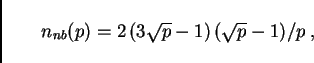
We also show data fits to the METIS curves,
![]() for the 200000 links network and
for the 200000 links network and
![]() for the 20024 links network, where
for the 20024 links network, where
![]() is the number of domains. We are not aware of any theoretical
argument for the shapes of these curves for METIS. It is however easy
to see that, for orthogonal bisection, the scaling of
is the number of domains. We are not aware of any theoretical
argument for the shapes of these curves for METIS. It is however easy
to see that, for orthogonal bisection, the scaling of ![]() has to
be
has to
be ![]() . Also, the limiting case where each node is on a
different CPU needs to have the same
. Also, the limiting case where each node is on a
different CPU needs to have the same ![]() both for bisection and
for METIS. In consequence, it is plausible to use a scaling form of
both for bisection and
for METIS. In consequence, it is plausible to use a scaling form of
![]() with
with ![]() . This is confirmed by the straight
line for large
. This is confirmed by the straight
line for large ![]() in the log-log-plot of Fig. 6.
Since for
in the log-log-plot of Fig. 6.
Since for ![]() , the number of split links
, the number of split links ![]() should be zero,
for the 20024 links network we use the equation
should be zero,
for the 20024 links network we use the equation
![]() , resulting in
, resulting in
![]() . For
the 200000 links network, the resulting fit is so bad
that we did not add the negative term. This leads to a kink for the
corresponding curves in Fig. 13.
. For
the 200000 links network, the resulting fit is so bad
that we did not add the negative term. This leads to a kink for the
corresponding curves in Fig. 13.
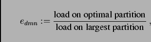
Such an investigation also allows to compute the theoretical
efficiency based on the graph partitioning. Efficiency is optimal if
each CPU gets exactly the same computational load. However, because
of the granularity of the entities (nodes plus attached half-links)
that we distribute, load imbalances are unavoidable, and they become
larger with more CPUs. We define the resulting theoretical efficiency
due to the graph partitioning as
![\includegraphics[width=\textwidth]{splitedges-gpl.eps}](img29.png)
|
![\includegraphics[width=\textwidth]{efficiency-e2-gpl.eps}](img31.png)
![\includegraphics[width=\textwidth]{efficiency-allstr-gpl.eps}](img32.png)
|
In the last section, we explained how the street network is partitioned into domains that can be loaded onto different CPUs. In order to be efficient, the loads on different CPUs should be as similar as possible. These loads do however depend on the actual vehicle traffic in the respective domains. Since we are doing iterations, we are running similar traffic scenarios over and over again. We use this feature for an adaptive load balancing: During run time we collect the execution time of each link and each intersection (node). The statistics are output to file. For the next run of the micro-simulation, the file is fed back to the partitioning algorithm. In that iteration, instead of using the link lengths as load estimate, the actual execution times are used as distribution criterion. Fig. 9 shows the new domains after such a feedback (compare to Fig. 5).
To verify the impact of this approach we monitored the execution times per time-step throughout the simulation period. Figure 10 depicts the results of one of the iteration series. For iteration 1, the load balancer uses the link lengths as criterion. The execution times are low until congestion appears around 7:30 am. Then, the execution times increase fivefold from 0.04 sec to 0.2 sec. In iteration 2 the execution times are almost independent of the simulation time. Note that due to the equilibration, the execution times for early simulation hours increase from 0.04 sec to 0.06 sec, but this effect is more than compensated later on.
The figure also contains plots for later iterations (11, 15, 20, and 40). The improvement of execution times is mainly due to the route adaptation process: congestion is reduced and the average vehicle density is lower. On the machine sizes where we have tried it (up to 16 CPUs), adaptive load balancing led to performance improvements up to a factor of 1.8. It should become more important for larger numbers of CPUs since load imbalances have a stronger effect there.
[width=]load-feedback.bw-gz.eps
|
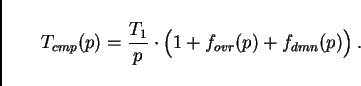
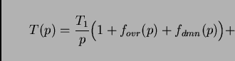
It is possible to systematically predict the performance of parallel micro-simulations (e.g. [20,27]). For this, several assumptions about the computer architecture need to be made. In the following, we demonstrate the derivation of such predictive equations for coupled workstations and for parallel supercomputers.
The method for this is to systematically calculate the wall clock time
for one time step of the micro-simulation. We start by assuming that
the time for one time step has contributions from computation,
![]() , and from communication,
, and from communication, ![]() . If these do not
overlap, as is reasonable to assume for coupled workstations, we have
. If these do not
overlap, as is reasonable to assume for coupled workstations, we have
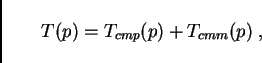 |
(2) |
Time for computation is assumed to follow
Time for communication typically has two contributions: Latency and
bandwidth. Latency is the time necessary to initiate the
communication, and in consequence it is independent of the message
size. Bandwidth describes the number of bytes that can be
communicated per second. So the time for one message is
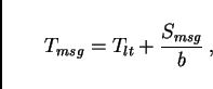
However, for many of today's computer architectures, bandwidth is given by at least two contributions: node bandwidth, and network bandwidth. Node bandwidth is the bandwidth of the connection from the CPU to the network. If two computers communicate with each other, this is the maximum bandwidth they can reach. For that reason, this is sometimes also called the ``point-to-point'' bandwidth.
The network bandwidth is given by the technology and topology of the network. Typical technologies are 10 Mbit Ethernet, 100 Mbit Ethernet, FDDI, etc. Typical topologies are bus topologies, switched topologies, two-dimensional topologies (e.g. grid/torus), hypercube topologies, etc. A traditional Local Area Network (LAN) uses 10 Mbit Ethernet, and it has a shared bus topology. In a shared bus topology, all communication goes over the same medium; that is, if several pairs of computers communicate with each other, they have to share the bandwidth.
For example, in our 100 Mbit FDDI network (i.e. a network bandwidth
of ![]() Mbit) at Los Alamos National Laboratory, we found
node bandwidths of about
Mbit) at Los Alamos National Laboratory, we found
node bandwidths of about ![]() Mbit. That means that two
pairs of computers could communicate at full node bandwidth, i.e.
using 80 of the 100 Mbit/sec, while three or more pairs were limited
by the network bandwidth. For example, five pairs of computers could
maximally get
Mbit. That means that two
pairs of computers could communicate at full node bandwidth, i.e.
using 80 of the 100 Mbit/sec, while three or more pairs were limited
by the network bandwidth. For example, five pairs of computers could
maximally get ![]() Mbit/sec each.
Mbit/sec each.
A switched topology is similar to a bus topology, except that the network bandwidth is given by the backplane of the switch. Often, the backplane bandwidth is high enough to have all nodes communicate with each other at full node bandwidth, and for practical purposes one can thus neglect the network bandwidth effect for switched networks.
If computers become massively parallel, switches with enough backplane
bandwidth become too expensive. As a compromise, such supercomputers
usually use a communications topology where communication to
``nearby'' nodes can be done at full node bandwidth, whereas global
communication suffers some performance degradation. Since we
partition our traffic simulations in a way that communication is
local, we can assume that we do communication with full node bandwidth
on a supercomputer. That is, on a parallel supercomputer, we can
neglect the contribution coming from the ![]() -term. This
assumes, however, that the allocation of street network partitions to
computational nodes is done in some intelligent way which maintains
locality.
-term. This
assumes, however, that the allocation of street network partitions to
computational nodes is done in some intelligent way which maintains
locality.
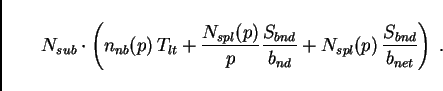
As a result of this discussion, we assume that the communication
time per time step is
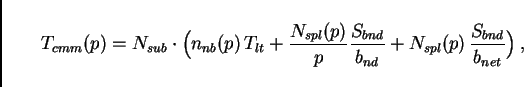
![]() is the number of neighbor domains each CPU talks to. All
information which goes to the same CPU is collected and sent as a
single message, thus incurring the latency only once per neighbor
domain. For
is the number of neighbor domains each CPU talks to. All
information which goes to the same CPU is collected and sent as a
single message, thus incurring the latency only once per neighbor
domain. For ![]() ,
, ![]() is zero since there is no other domain to
communicate with. For
is zero since there is no other domain to
communicate with. For ![]() , it is one. For
, it is one. For ![]() and
assuming that domains are always connected, Euler's theorem for planar
graphs says that the average number of neighbors cannot become more
than six. Based on a simple geometric argument, we use
and
assuming that domains are always connected, Euler's theorem for planar
graphs says that the average number of neighbors cannot become more
than six. Based on a simple geometric argument, we use
![]() is the latency (or start-up time) of each message.
is the latency (or start-up time) of each message. ![]() between 0.5 and 2 milliseconds are typical values for PVM on a
LAN [34,12].
between 0.5 and 2 milliseconds are typical values for PVM on a
LAN [34,12].
Next are the terms that describe our two bandwidth effects.
![]() is the number of split links in the whole simulation;
this was already discussed in Sec. 6 (see
Fig. 6). Accordingly,
is the number of split links in the whole simulation;
this was already discussed in Sec. 6 (see
Fig. 6). Accordingly, ![]() is the number
of split links per computational node.
is the number
of split links per computational node. ![]() is the size of
the message per split link.
is the size of
the message per split link. ![]() and
and ![]() are the
node and network bandwidths, as discussed above.
are the
node and network bandwidths, as discussed above.
In consequence, the combined time for one time step is
According to what we have discussed above, for ![]() the
number of neighbors scales as
the
number of neighbors scales as
![]() and the number of
split links in the simulation scales as
and the number of
split links in the simulation scales as
![]() . In consequence for
. In consequence for ![]() and
and ![]() small enough,
we have:
small enough,
we have:
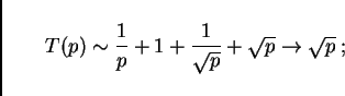
The curves in Fig. 11 are results from this
prediction for a switched 100 Mbit Ethernet LAN; dots and crosses show
actual performance results. The top graph shows the time for one time
step, i.e. ![]() , and the individual contributions to this value.
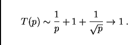
The bottom graph shows the real time ratio (RTR)
, and the individual contributions to this value.
The bottom graph shows the real time ratio (RTR)
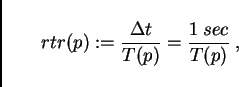
The plot (Fig. 11) shows that even something as relatively profane as a combination of regular Pentium CPUs using a switched 100Mbit Ethernet technology is quite capable in reaching good computational speeds. For example, with 16 CPUs the simulation runs 40 times faster than real time; the simulation of a 24 hour time period would thus take 0.6 hours. These numbers refer, as said above, to the Portland 20024 links network. Included in the plot (black dots) are measurements with a compute cluster that corresponds to this architecture. The triangles with lower performance for the same number of CPUs come from using dual instead of single CPUs on the computational nodes. Note that the curve levels out at about forty times faster than real time, no matter what the number of CPUs. As one can see in the top figure, the reason is the latency term, which eventually consumes nearly all the time for a time step. This is one of the important elements where parallel supercomputers are different: For example the Cray T3D has a more than a factor of ten lower latency under PVM [12].
As mentioned above, we also ran the same simulation without any vehicles. In the TRANSIMS-1999 implementation, the simulation sends the contents of each CA boundary region to the neighboring CPU even when the boundary region is empty. Without compression, this is five integers for five sites, times the number of lanes, resulting in about 40 bytes per split edge, which is considerably less than the 800 bytes from above. The results are shown in Fig. 12. Shown are the computing times with 1 to 15 single-CPU slaves, and the corresponding real time ratio. Clearly, we reach better speed-up without vehicles than with vehicles (compare to Fig. 11). Interestingly, this does not matter for the maximum computational speed that can be reached with this architecture: Both with and without vehicles, the maximum real time ratio is about 80; it is simply reached with a higher number of CPUs for the simulation with vehicles. The reason is that eventually the only limiting factor is the network latency term, which does not have anything to do with the amount of information that is communicated.
Fig. 13 (top) shows some predicted real time ratios for other computing architectures. For simplicity, we assume that all of them except for one special case explained below use the same 500 MHz Pentium compute nodes. The difference is in the networks: We assume 10 Mbit non-switched, 10 Mbit switched, 1 Gbit non-switched, and 1 Gbit switched. The curves for 100 Mbit are in between and were left out for clarity; values for switched 100 Mbit Ethernet were already in Fig. 11. One clearly sees that for this problem and with today's computers, it is nearly impossible to reach any speed-up on a 10 Mbit Ethernet, even when switched. Gbit Ethernet is somewhat more efficient than 100 Mbit Ethernet for small numbers of CPUs, but for larger numbers of CPUs, switched Gbit Ethernet saturates at exactly the same computational speed as the switched 100 Mbit Ethernet. This is due to the fact that we assume that latency remains the same - after all, there was no improvement in latency when moving from 10 to 100 Mbit Ethernet. FDDI is supposedly even worse [12].
The thick line in Fig. 13 corresponds to the ASCI Blue Mountain parallel supercomputer at Los Alamos National Laboratory. On a per-CPU basis, this machine is slower than a 500 MHz Pentium. The higher bandwidth and in particular the lower latency make it possible to use higher numbers of CPUs efficiently, and in fact one should be able to reach a real time ratio of 128 according to this plot. By then, however, the granularity effect of the unequal domains (Eq. (1), Fig. 8) would have set in, limiting the computational speed probably to about 100 times real time with 128 CPUs. We actually have some speed measurements on that machine for up to 96 CPUs, but with a considerably slower code from summer 1998. We omit those values from the plot in order to avoid confusion.
Fig. 13 (bottom) shows predictions for the higher
fidelity Portland 200000 links network with the same
computer architectures. The assumption was that the time for one time
step, i.e. ![]() of Eq. (3), increases by a factor of
eight due to the increased load. This has not been verified yet.
However, the general message does not depend on the particular
details: When problems become larger, then larger numbers of CPUs
become more efficient. Note that we again saturate, with the switched
Ethernet architecture, at 80 times faster than real time, but this
time we need about 64 CPUs with switched Gbit Ethernet in order to get
40 times faster than real time -- for the smaller Portland
20024 links network with switched Gbit Ethernet we would
need 8 of the same CPUs to reach the same real time ratio. In short
and somewhat simplified: As long as we have enough CPUs, we can
micro-simulate road networks of arbitrarily largesize, with
hundreds of thousands of links and more, 40 times faster than real
time, even without supercomputer hardware. -- Based on our
experience, we are confident that these predictions will be lower
bounds on performance: In the past, we have always found ways to make
the code more efficient.
of Eq. (3), increases by a factor of
eight due to the increased load. This has not been verified yet.
However, the general message does not depend on the particular
details: When problems become larger, then larger numbers of CPUs
become more efficient. Note that we again saturate, with the switched
Ethernet architecture, at 80 times faster than real time, but this
time we need about 64 CPUs with switched Gbit Ethernet in order to get
40 times faster than real time -- for the smaller Portland
20024 links network with switched Gbit Ethernet we would
need 8 of the same CPUs to reach the same real time ratio. In short
and somewhat simplified: As long as we have enough CPUs, we can
micro-simulate road networks of arbitrarily largesize, with
hundreds of thousands of links and more, 40 times faster than real
time, even without supercomputer hardware. -- Based on our
experience, we are confident that these predictions will be lower
bounds on performance: In the past, we have always found ways to make
the code more efficient.
![\includegraphics[width=0.8\hsize]{cars-time-gpl.eps}](img78.png)
![\includegraphics[width=0.8\hsize]{cars-rtr-gpl.eps}](img79.png)
|
![\includegraphics[width=0.8\hsize]{nocars-time-gpl.eps}](img80.png)
![\includegraphics[width=0.8\hsize]{nocars-rtr-gpl.eps}](img81.png)
|
![\includegraphics[width=0.8\hsize]{other-rtr-gpl.eps}](img82.png)
![\includegraphics[width=0.8\hsize]{ten-rtr-gpl.eps}](img83.png)
|
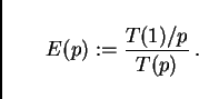
We have cast our results in terms of the real time ratio, since this is the most important quantity when one wants to get a practical study done. In this section, we will translate our results into numbers of speed-up, efficiency, and scale-up, which allow easier comparison for computing people.
Let us define speed-up as
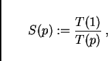
Now note again that the real time ratio is
![]() Thus, in order to obtain the speed-up from the real time ratio, one
has to multiply all real time ratios by
Thus, in order to obtain the speed-up from the real time ratio, one
has to multiply all real time ratios by ![]() . On a
logarithmic scale, a multiplication corresponds to a linear shift. In
consequence, speed-up curves can be obtained from our real time ratio
curves by shifting the curves up or down so that they start at one.
. On a
logarithmic scale, a multiplication corresponds to a linear shift. In
consequence, speed-up curves can be obtained from our real time ratio
curves by shifting the curves up or down so that they start at one.
This also makes it easy to judge if our speed-up is linear or not.
For example in Fig. 13 bottom, the curve which starts
at 0.5 for 1 CPU should have an RTR of 2 at 4 CPU, an RTR of 8 at
16 CPUs, etc. Downward deviations from this mean sub-linear speed-up.
Such deviations are commonly described by another number, called
efficiency, and defined as
![\includegraphics[width=0.8\hsize]{eff-gpl.eps}](img91.png)
|
As explained in the introduction, a micro-simulation in a software suite for transportation planning would have to be run many times (``feedback iterations'') in order to achieve consistency between modules. For the microsimulation alone, and assuming our 16 CPU-machine with switched 100 Mbit Ethernet, we would need about 30 hours of computing time in order to simulate 24 hours of traffic fifty times in a row. In addition, we have the contributions from the other modules (routing, activities generation). In the past, these have never been a larger problem than the micro-simulation, for several reasons:
This paper explains the parallel implementation of the TRANSIMS micro-simulation. Since other modules are computationally less demanding and also simpler to parallelize, the parallel implementation of the micro-simulation is the most important and most complicated piece of parallelization work. The parallelization method for the TRANSIMS micro-simulation is domain decomposition, that is, the network graph is cut into as many domains as there are CPUs, and each CPU simulates the traffic on its domain. We cut the network graph in the middle of the links rather than at nodes (intersections), in order to separate the traffic dynamics complexity at intersections from the complexity of the parallel implementation. We explain how the cellular automata (CA) or any technique with a similar time depencency scheduling helps to design such split links, and how the message exchange in TRANSIMS works.
The network graph needs to be partitioned into domains in a way that the time for message exchange is minimized. TRANSIMS uses the METIS library for this goal. Based on partitionings of two different networks of Portland (Oregon), we calculate the number of CPUs where this approach would become inefficient just due to this criterion. For a network with 200000 links, we find that due to this criterion alone, up to 1024 CPUs would be efficient. We also explain how the TRANSIMS micro-simulation adapts the partitions from one run to the next during feedback iterations (adaptive load balancing).
We finally demonstrate how computing time for the TRANSIMS micro-simulation (and therefore for all of TRANSIMS) can be systematically predicted. An important result is that the Portland 20024 links network runs about 40 times faster than real time on 16 dual 500 MHz Pentium computers connected via switched 100 Mbit Ethernet. These are regular desktop/LAN technologies. When using the next generation of communications technology, i.e. Gbit Ethernet, we predict the same computing speed for a much larger network of 200000 links with 64 CPUs.
This is a continuation of work that was started at Los Alamos National Laboratory (New Mexico) and at the University of Cologne (Germany). An earlier version of some of the same material can be found in Ref. [36]. We thank the U.S. Federal Department of Transportation and Los Alamos National Laboratory for making TRANSIMS available free of charge to academic institutions. The version used for this work was ``TRANSIMS-LANL Version 1.0''.
~karypis/metis/metis.html.
~mr/dissertation.
This document was generated using the LaTeX2HTML translator Version 2K.1beta (1.47)
Copyright © 1993, 1994, 1995, 1996,
Nikos Drakos,
Computer Based Learning Unit, University of Leeds.
Copyright © 1997, 1998, 1999,
Ross Moore,
Mathematics Department, Macquarie University, Sydney.
The command line arguments were:
latex2html -split 1 -dir html parallel.tex
The translation was initiated by Kai Nagel on 2001-07-01
![\includegraphics[width=\hsize]{bnd-gz.eps}](img13.png)
![\includegraphics[width=\hsize]{ob-plot-gpl.eps}](img28.png)
![\includegraphics[width=\hsize]{metis-plot-gpl.eps}](img30.png)
![\includegraphics[width=\hsize]{ob-fb-plot-gpl.eps}](img33.png)