Parallel Queue Model Approach to Traffic Microsimulations

Nurhan Cetin¹,   Kai Nagel²
Dept. of Computer Science, ETH Zürich, 8092 Zürich,
Switzerland

Abstract:

In this paper, we explain a parallel implementation of a traffic micro-simulation model based on the queue model introduced by Gawron. Within this model, links do not only have a flow capacity that limits the number of vehicles that can leave the link, but also have a space constraint which limits the number of vehicles that can be on a link simultaneously. The vehicles in this model follow their precomputed paths as in other route-plan-based simulations such as TRANSIMS. Since the queue model needs less data and computing power, it runs much faster than TRANSIMS for the same data. In the parallel implementation of the queue model we distribute the data onto a number of processors, each of which runs a smaller portion of the simulation. The parallel version gives a runtime that is 100 times faster than real time. We test this simulation on a scenario using the road network of Switzerland.

Keywords: Traffic Simulation, Queue Model, Parallel Programming, MPI

Introduction

Queueing theory is the study of systems of queues where items arrive to the queues for service, wait in the queues for a while, receive service from one or more servers, and leave. Queues, i.e, waiting lines, form because resources are limited. Queueing theory deals with problems which involve waiting lines, i.e, it handles the problems of congestion.

Queueing theory studies the issues such as the rate of arrivals at the queue, the average waiting time until being served, the average queue length, etc., by knowing arrival rates and service rates. Queues in a system have a certain service rate. If the arrival rate of the items is greater than the service rate, queues are created to keep the excessive arrivals.

In this paper, we model traffic based on an extended version of queueing theory. We will use the term ``Queue Model'' instead of the term ``Queueing Theory'' in order to stress those extensions. Our aim is to simulate the links as queues and to make the intersection logic realistic.

In queueing theory, it is usual to define queues of infinite length. If the capacity of a queue is finite, queueing theory defines the system loss as follows: If a new item arrives to a queue which does not have any empty space, then the item leaves without being served (the item is called ``lost''). In our case, instead of losing the item, we refuse to accept it, which means that it does not get served at the upstream server even if the server has free capacity. Since this behavior can cause deadlocks (loops of completely congested queues), we remove vehicles from the simulation if they have not moved for a certain amount of time. Our goal, however, is to have a simulation which does not lose any items.

The paper is organized as follows: Implementation of queue model is explained in section 2. Section 3 gives an introduction to parallel programming. Parallel implementation of the queue model is given in Section 4. Section 5 discusses the simulation results.

Queue Model

In our model, the streets (links) are represented by finite queues. The dynamics of the queue model described and implemented here focus on two main reasons of a congestion. The first of these reasons is defined by not allowing more vehicles to leave a link per time step than the number of vehicles that are allowed to leave according to the link's capacity. This is the capacity constraint. The second one is that links can only store a certain number of vehicles, which we call the storage constraint. The storage constraint causes queue spill-back, and it reduces the number of incoming vehicles to the link once a link is full.

In consequence, each link is represented by a queue with a free flow velocity $v_{0}$, a length $L$, a capacity $C$ and a number of lanes $n_{lanes}$. Free flow velocity is the velocity of a car when the traffic density is very low such that a car can go through that particular link as fast as possible. Free flow travel time is calculated by .

The storage constraint of a link is calculated as , where $l_{sites}$ is the space a single vehicle in the average occupies in a jam, which is the inverse of the jam density. We use $l_{sites} = 7.5 \hbox{m}$. The flow capacity, on the other hand, is given by the input files.

As mentioned above, vehicles in the simulation can get stuck if congested links form a closed loop, and the vehicles at the downstream end of each of these links want to move into the next of these full links. In order to prevent this gridlock, any vehicle at the beginning of a queue that has not moved for over 300 simulation time steps (seconds) is removed from the simulation.

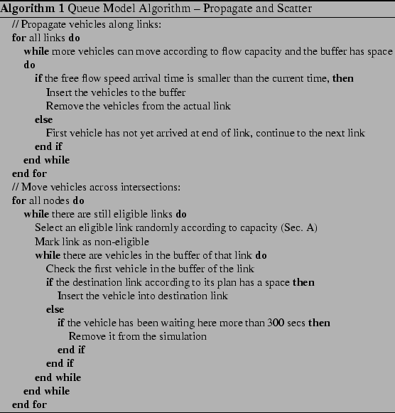
The queue model is implemented using the algorithm shown in Alg. 1. The algorithm given there is based on the algorithm described in [1,6] but with a modified intersection dynamics. In those references, the intersection logic essentially is:

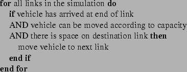
The three conditions mean the following:

• A vehicle that enters link $a$ at time $t_0$ cannot leave the link before time $t_0 + T_0$, as explained above.

• The condition ``vehicle can be moved according to capacity'' is determined as
  
  $$\Big(N_{link}  <  int(C_{link})\Big)  OR  \Big(N_{link} = int(C_{link})  AND   rnd  <  C_{link}-int(C_{link})\Big)$$
  
  
  where $C_{link}$ is the capacity of the link and $N_{link}$ is the number of the vehicles which already left the same link in the same time step. $rnd$ is a random number such that $0\leq rnd \leq 1$ and $int(x)$ returns the integer part of the number $x$. What it is meant by this formula is that the vehicles can leave the link if leaving capacity of the link has not been exceeded yet in this time step. If the capacity per time step is non-integer, then we move the last vehicle with a probability which is equal to the non-integer part of the capacity per time step.

• ``space on destination link'' is the important difference to standard queue models: If the destination link is full, the vehicle will not move across the intersection.

The problem with this algorithm is that links are always selected in the same sequence, thus giving some links a higher priority than others under congested conditions. Note that the ``winning'' link is not the link which is earliest in the sequence, but the link which is first after when traffic on the destination link has moved.

Simple randomization of the link sequence is only a partial remedy since what one truly wants is to give links with a higher capacity also a higher priority. In consequence, we have modified the algorithm so that links are prioritized randomly according to capacity. That is, links with high capacity are more often first than links with low capacity. At the same time, we have moved the algorithm from link-oriented to intersection-oriented (that is, the loop now goes over all intersections, which then look at all incoming links), and we have separated the capacity constraint from the intersection logic. The last was done by introducing a separate buffer at the end of the link, which is of size $\lceil C_{link} \rceil$, i.e. the first integer number being larger or equal than the link capacity (in vehicles per time step). Vehicles are then moved from the link into the buffer according to the capacity constraint and only if there is space in the buffer; once in the buffer, vehicles can be moved across intersections without looking at the capacity constraints.

The above details are given in algorithmic form in Alg. 1. In addition and in preparation for parallel computing, we have made the dynamics of the algorithm completely parallel. What this means is that, if traffic is moved out of a full link, the new empty space will not become available until the next time step - at which time it will be shared between the incoming links according to the method described above. This has the advantage that all information which is necessary for the computation of a time step is available locally at each intersection before the time step starts - and in consequence there is no information exchange between intersections during the computation of the time step.

Figure 1: Link dynamics with buffer

Parallel Computing

General Issues

The idea behind parallel computing is that a task can be achieved faster if it is divided into a set of subtasks each of which is assigned to a different processor. The aim is to speed up the computation as a whole.

A possible parallel computation environment is for example a cluster of standard Pentium computers, coupled via standard 100 Mbit Ethernet LAN. Each computer would then get a subtask as described above.

In order to generate a parallel program, one must think about (i) how to partition the tasks into subtasks, (ii) how to provide the data exchange between the subtasks. One possibility of partitioning is to decompose the task so that each subtask can run the same program on a smaller portion of data independent of the other subtasks. When a subtasks needs information/data from another subtask, then communication is required.

As an example, a traffic simulation might take a long time to run if the underlying network is large and the number of vehicles is high. If one cares about fast computation time, then parallel computing is a solution since it solves the problem cost-effectively by aggregating the power and memory of many computers. What needs to be done is to partition the street network and to distribute the vehicles according to the partitioning information. If a vehicle needs to move into a link which is on an another partition, then a communication between these two partitions takes place.

Partitioning of a domain can be done in several ways. Finding the best way of doing a decomposition depends on what is to be decomposed. In our traffic simulation, we need to divide the network (of the streets and the intersections) into a number of subnetworks. In order to achieve this, we use a software package called METIS  [2] which is based on multilevel graph partitioning. After the partitioning is done, each processor is assigned to a subpart.

With respect to communication, there are in general two main approaches to inter-processor communication. One of them is called message passing between processors; its alternative is to use shared-address space where variables are kept in a common pool where they are globally available to all processors. Each paradigm has its own advantages and disadvantages.

In the shared-address space approach, all variables are globally accessible by all processors. Despite multiple processors operating independently, they share the same memory resources. Accessing the memory should be provided in a mutually exclusive fashion since accesses to the same variable at the same time by multiple processors might lead to inconsistent data. Shared-address space approach makes it simpler for the user to achieve parallelism but since the memory bandwidth is limited, severe bottlenecks are unavoidable with the increasing number of processors, or alternatively such shared memory parallel computers become very expensive. Also, the user is responsible for providing the synchronization constructs in order to provide concurrent accesses.

In the message passing approach, there are independent cooperating processors. Each processor has a private local memory in order to keep the variables and data, and thus can access local data very rapidly. If an exchange of the information is needed between the processors, the processors communicate and synchronize by passing messages which are simple send and receive instructions. Message passing can be imagined similar to sending a letter. The following phases happen during a message passing operation.

1. The message needs to be packed. Here, one tells the computer which data needs to be sent.

2. The message is sent away.

3. The message then may take some time on the network until it finally arrives in the receiver's inbox.

4. The receiver has to officially receive the message, i.e. to take it out of the inbox.

5. The receiver has to unpack the message and tell the computer where to store the received data.

There are time delays associated with each of these phases. It is important to note that some of these time delays are incurred even for an empty message (``latency''), whereas others depend on the size of the message (``bandwidth restriction''). We will come back to this in the next section.

The communication among the processors can be achieved by using a message passing library which provides the functions to send and receive data. There are several libraries such as MPI [3] (Message Passing Interface) or PVM [5] (Parallel Virtual Machine) for this purpose. Both PVM and MPI are software packages/libraries that allow heterogeneous PCs interconnected by a network to exchange data. They both define an interface for the different programming languages such as C/C++ or Fortran. For the purposes of parallel traffic simulation, the differences between PVM and MPI are negligible; we use MPI since it has slightly more focus on computational performance.

Performance Issues

The size of input usually determines the performance of a sequential algorithm (or program) evaluated in terms of execution time. However, this is not the case for the parallel programs. When evaluating parallel programs, besides the input size, the computer architecture and also the number of the processors must be taken into consideration.

There are various metrics to evaluate the performance of a parallel program. Execution time, Speedup and Efficiency are the most common metrics to measure the performance of a parallel program. We will discuss these metrics in the following subsections.

Execution Time

The execution time of a parallel program is defined as the total time elapsed from the time the first processor starts execution to the time the last processor completes the execution. During execution, a processor is either computing or communicating. Therefore,

$$T(p) = T_{cmp}(p) + T_{cmm}(p) ,$$

where $T$ is the execution time, $p$ is the number of processors, $T_{cmp}$ is the computation time and $T_{cmm}$ is the communication time.

For traffic simulation, the time required for the computation, namely, $T_{cmp}$ can be calculated roughly in terms of the serial execution time (run time of the algorithm on a single CPU) divided by the number of processors. Thus,

$$T_{cmp}(p) \approx {T_1 \over p} ,$$

where $T_{1}$is the serial execution time, $p$ is the number of CPUs. More exact formulas would also contain the overhead effects and unequal domain size effects.

As mentioned above, time for communication typically has two contributions: Latency and bandwidth. Latency is the time necessary to initiate the communication i.e, the message size has no effect here. Bandwidth describes the number of bytes that can be exchanged per second. So the time for one message is

$$T_{msg} = T_{lt} + {S_{msg} \over b} ,$$

where $T_{lt}$ is the latency, $S_{msg}$ is the message size, and $b$ is the bandwidth.

Speed-Up

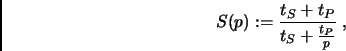
Maybe the most useful metric in measuring performance of a parallel program is how much performance gain is achieved by the program. Speedup achieved by a parallel algorithm is defined as the ratio of the time required by the best sequential algorithm to solve a problem, $T(1)$, to the time required by parallel algorithm using $p$ processors to solve the same problem, $T(p)$:

$$S(p) := {T(1) \over T(p)} .$$

Depending on the viewpoint, for $T(1)$ one uses either the running time of the parallel algorithm on a single CPU, or the fastest existing sequential algorithm. In our model, we measure the serial execution time by running the parallel program only one CPU.

Speedup is limited by a couple of factors. First, the software overhead appears in the parallel implementation since the parallel functionality requires additional lines of code. Second, speedup is generally limited by the speed of the slowest node or processor. Thus, we need to make sure that each node performs the same amount of work. i.e. the system is load balanced. Third, if the communication and computation cannot be overlapped, then the communication will reduce the speed of the overall application.

A final limitation of the speedup is known as Amdahl's Law - Serial Fraction. This states that the speedup of a parallel algorithm is effectively limited by the number of operations which must be performed sequentially. Thus, let us define, for a sequential program, $t_{S}$ as the amount of the time spent by one processor on sequential parts of the program and $t_{P}$ as the amount of the time spent by one processor on parts of the program that can be parallelized. Then, we can formulate the serial run-time as $T(1) := t_{S} + t_{P}$ and the parallel run-time as $T(p) := t_{S} + t_{P}/p$.

Therefore, the serial fraction $F$ will be

$$F := { t_{S} \over T(1)} ,$$

and the speedup $S(p)$ is expressed as

$$S(p) := {{t_{S} + t_{P}} \over {t_{S} + {{t_{P}} \over{p}}}} ,$$

or in terms of serial fraction, it would be

$$S(p) := {{1} \over {F + {{1 - F} \over{p}}}} .$$

This means that even for $p \to \infty$, the speedup can be no larger than $1/F$.

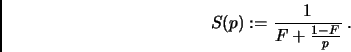
As an illustration, let us say, we have a program of which 80% can be done in parallel and 20% must be done sequentially. Then even for $p \to \infty$, we have $S(p) = 1/F = 5$, meaning that even with an infinite number of processors we are no more than 5 times faster than we were with a single processor.

Efficiency

An ideal system with ${p}$ processors might have a speedup up to ${p}$. However, this is not the case in practice since, as pointed out above, some parts of the program cannot be parallelized efficiently. Also, processors will spend time on communication. Efficiency is defined as

$$E(p) = \frac{S(p)}{p} .$$

Efficiency is a measure of the percentage of time for which a parallel computer with $p$ processors is utilized effectively. Ideally, efficiency equals to 1 but in practice, it is between 0 and 1 depending on how a processor is employed. This number is particularly useful when the overall execution time does not matter but one is interested in efficient hardware usage.

Parallel Queue Model

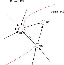
The decomposition at the boundaries of the subnetworks in our simulation is shown in Figure 2. Each node has outgoing and incoming links. As shown in Figure , the nodes at the boundaries are divided in a way that the nodes and the incoming links of those nodes are on the same processor.

Figure 2: Communication between nodes in the boundaries: Node N1 needs to communicate with N2 and N3. Since N2 and N3 are on the same processor, they do not need to establish a communication between themselves.

Whenever a vehicle is at the boundary of a processor and needs to go to a link which is located on another processor, the vehicle is sent to that other processor by using message passing. The neighbor processor receives the vehicle and inserts it into the appropriate link.

There is actually another parallel communication step which is necessary before the intersection dynamics is run. In that communication step, each link sends its number of empty spaces to its from-node, i.e. the node where it is an outgoing link. If link and node are on the same processor, this is a simple data copy operation; if they are on different processors, then this involves a send and receive. The resulting parallel algorithm is given as Alg. 2.

In order to run our parallel application, we run it on a cluster of 32 Pentium PCs connected by 100 Mbit Ethernet, which is a standard LAN technology. The PCs run Linux as an operating system. Using a supercomputer such as IBM SP2 or Intel iPSC/860 in order to achieve the parallelism is more expensive and not necessarily faster.

With respect to domain decomposition, Fig.  shows a result of using the METIS default routine called kmetis. Experimenting with other METIS options did not lead to any improvement. An important reason for this is that the default options of METIS-4.0, which reduce the number of neighboring processors one needs to communicate with, are exactly what we need for our Beowulf cluster architecture.

Figure 3: Decomposition of the Switzerland street network. Each color corresponds to a different processor.

Simulation results for Switzerland

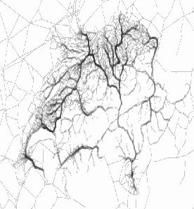
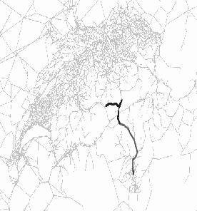
A so-called Gotthard scenario is a test for our simulations. In this scenario, we have a set of 50000 trips going to the same destination. Having all trips going to the same destination allows us to check the traffic jams on all used routes to the destination.

More specifically, the 50'000 trips have random starting points all over Switzerland, a random starting time between 6am and 7am, and they all go to Lugano. In order for the vehicles to get there, many of them should go through the Gotthard Tunnel. Thus, there are traffic jams at the beginning of Gotthard Tunnel, specifically on the highways coming from Schwyz and Luzern. This scenario has some similarity with vacation traffic in Switzerland.

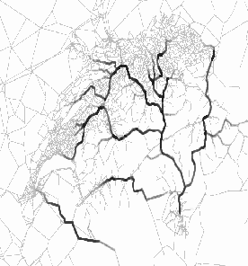
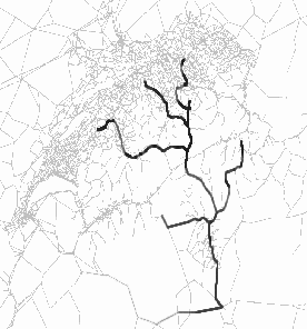
Some snapshots can be viewed in Figure 4. The links with higher densities are indicated by darker pixels. Thus, the darker colored links are where the traffic jams are. The top left picture shows the case at 6:30am. As can be seen, the traffic is all over Switzerland. Therefore, there are not many congested links. In the top right figure, we see traffic at 7:30am where the vehicles are moving towards the highways. Since the vehicles coming from different towns are moving into the same highways, congestion is unavoidable and it is shown as the darker pixels.

The figure on the bottom left is the snapshot at 9:45am where most of the vehicles are on the main highways. In the bottom right snapshot, the simulation is near the end. The vehicles, that have passed through the Gotthard Tunnel, continue to Lugano and exit the simulation there. The Gotthard Tunnel and its immediate upstream links are indicated by darker pixels almost all the time except at the very beginning of the simulation.

Figure 4: Snapshots from the visualizer. Vehicles are moving towards to Lugano.

Table 1 shows computing speeds for different numbers of CPUs for the queue simulation. This table shows the performance of the queue micro-simulation on a Beowulf Pentium cluster. The second column gives the number of seconds taken to run the first 3 hours of the Gotthard scenario. The third column gives the real time ratio (RTR), which is how much faster than reality the simulation is. A RTR of 100 means that one simulates 100 seconds of the traffic scenario in one second of wall clock time.

Table 1: Computational performance on a Beowulf Pentium cluster. ``Q'' entries: queue simulation. ``TR'' entries: TRANSIMS (TRANSIMS performance data from [4]).

Number of Procs	Time elapsed Q	Real Time Ratio Q	Real Time Ratio TR
1	357	30.25	4.5
4	153	70.59	14.9
8	108	100.00	26.6
12	104	103.85
16	115	93.91	40.9
24	142	76.06
32	212	50.94

One could run larger scenarios at the same computational speed when using more CPUs. As the next step, we will be running our simulation on more realistic scenario which generates 10 million trips based on actual traffic patterns.

Acknowledgments

We would like to thank Andreas Völlmy for providing initial plan set data and Bryan Raney for the feedback he has given on this paper.

Selecting a link randomly according to capacity

Here is an algorithm which selects a link with a probability proportional to its capacity. It is a general algorithm which selects proportional to weight when faced with $N$ items with non-normalized weights $w_i$.

Bibliography

1

C. Gawron.
An iterative algorithm to determine the dynamic user equilibrium in a traffic simulation model.
International Journal of Modern Physics C, 9(3):393-407, 1998.

2

METIS library.
www-users.cs.umn.edu/~karypis/metis/.

3

MPI: Message Passing Interface.
See www-unix.mcs.anl.gov/mpi/mpich.

4

K. Nagel and M. Rickert.
Parallel implementation of the TRANSIMS micro-simulation.
Parallel Computing, 27(12):1611-1639, 2001.

5

PVM: Parallel Virtual Machine.
See www.epm.ornl.gov/pvm/pvm_home.html.

6

P. M. Simon and K. Nagel.
Simple queueing model applied to the city of Portland.
International Journal of Modern Physics C, 10(5):941-960, 1999.

About this document ...

Parallel Queue Model Approach to Traffic Microsimulations

This document was generated using the LaTeX2HTML translator Version 2K.1beta (1.47)

Copyright © 1993, 1994, 1995, 1996, Nikos Drakos, Computer Based Learning Unit, University of Leeds.
Copyright © 1997, 1998, 1999, Ross Moore, Mathematics Department, Macquarie University, Sydney.

The command line arguments were:
latex2html -split 1 -dir html ParallelQueueModel.tex

The translation was initiated by Kai Nagel on 2002-04-02