The stochastic traffic cellular automaton (STCA)

The CA introduced in Chap. 7 can be made more general by allowing vehicles to travel more than one cell per time step. Also, it makes the simulation more realistic and more robust against artifacts if one introduces some randomness. Both are achieved with the following update rules:

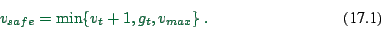
• Car-following rule:
  
  $$v_{safe} = \min \{ v_{t} + 1 , g_{t} , v_{max} \} \ .$$
  
  
  $g_t$ is the number of empty spaces to the car in front (``gap''); $v_{max}$ is the maximum velocity of the car under consideration.
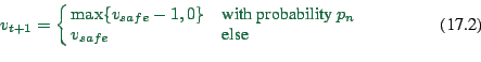
• Randomization:
  
  $$\displaystyle v_{t+1} = \cases{%% \max \{ v_{safe} - 1 , 0 \} & with probability $p_n$\ \cr v_{safe} & else \cr }$$
  
  

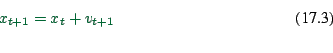
• Moving:
  
  $$x_{t+1} = x_{t} + v_{t+1}$$
  
  

$t$ and $t+1$ here refer to the actual time-steps of the simulation. The first rule describes deterministic car-following: try to accelerate by one velocity unit except when the gap is too small or when the maximum velocity is reached.

The second rule describes random noise: with probability $p_n$, a vehicle ends up being slower than calculated deterministically. This parameter simultaneously models three effects:

1. Speed fluctuations during free driving: Assume a vehicle with no other vehicles are nearby. It will eventually have speed $v_{max} -1$ or $v_{max}$. In both cases, $v_{safe}$ will be $v_{max}$. After the randomization, the speed will be at $v_{max} -1$ with probability $p_n$, and at $v_{max}$ else. That is, the speed of a single undisturbed vehicle fluctuates between $v_{max}$ and $v_{max} -1$.

2. Over-reactions at braking and car-following: Assume a vehicle with $v_{max}$ that approaches a slower vehicle from behind. Eventually, it will reach a gap 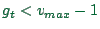$g_t < v_{max} - 1$. $v_{safe}$ will be equal to this $g_t$, and $v_{t+1}$ will either be equal to $g_t$ or one smaller (without becoming negative). That is, with probability $p_n$, the braking vehicle will not be at speed $g_t$ but slower.

   The argument for car following is similar: Assume a leading vehicle with speed $v_{lead} < v_{max}$. The follower will attempt to follow with $g_t = v_{lead}$ but in fact will fluctuate around that speed.

3. Randomness during acceleration: Assume a single vehicle with speed zero. Instead of acceleration $0\to1\to2\to3\to\ldots$, the acceleration will typically look like $0\to0\to1\to2\to2\to3\to\ldots$. Note that the rules are such that the velocity never decreases during acceleration.

Obviously, these effects overlap to a certain extent; for example, if $g_t = v_{max}$ one cannot say if $p_n$ refers to car following or to driving at free speed.

A translation into real-world units can be obtained as follows: The length $\ell$ of a cell is given by the average space a car occupies in a jam, since under jammed conditions each cell is filled by one car. Thus, $\ell = 1/\rho_{jam} \approx 7.5~m$. A simulation time step typically corresponds to one second in reality, and the order of magnitude of this can be justified by reaction time arguments (Sec. 27.4.1). One of the side-effects of this convention is that space can be measured in ``cells'' and time in ``time steps'', and usually these units are assumed implicitly and thus left out of the equations. A speed of, say, $v=5$, means that the vehicle travels five cells per time step, or 37.5 m/s, or 135 km/h, or approx. 85 mph.

$p_n$ is often set to $1/2$ for theoretical work, while for realistic traffic modelling $p_n = 0.2$ is a better choice.

[[would be possible to show this in validation (more fdiags, as function of params)]]