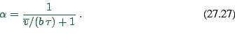
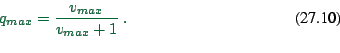
Any more realistic car micro-simulation first needs to have a method for simple car following. Such methods can be developed on single-lane loops, similar to a single-lane race track. A good way to start is the rule of thumb of ``two seconds time headway'', that many of us learn at driving school. We are supposed to have two seconds between the time when the car ahead passes a certain location, and the time when we pass it. The reason for this is related to our reaction time. If the car ahead starts braking really hard right when its back bumper is at that location, and if, after a reaction time, we start braking when our front bumper is at that same position, we will barely avoid a crash (see Fig. 27.3). Thus, time headway needs to be larger than reaction time, which translates into a space headway proportional to speed. As a consequence, most car following models have as their most important term one that makes the velocity a roughly linear function of the space headway or gap, although usually a reaction delay of one instead of two seconds is used.27.3 All car following models based on this principle have a similar dynamical behavior. For example, the transition from laminar to start-stop traffic is similar for all these models (67). Car following models which are used in micro-simulations are usually designed to be free of accidents.
![\includegraphics[width=0.5\hsize]{rct-time-fig.eps}](img351.png)
![\includegraphics[width=0.5\hsize]{rct-time-2-fig.eps}](img352.png)
|
Incarnations of car following can use continuous or discrete time, and continuous or discrete space. While continuous space and continuous time is more realistic, discrete space and time are more natural for a digital computer. And recent research has shown that, in the spirit of Statistical Physics, extremely simple and even unrealistic rules on the microscopic level can still lead to reasonable behavior on the macroscopic level (78,79,90,19,66). In consequence, cellular automata (CA) techniques, which are discrete in space and time, plus have a parallel local update, can actually simulate traffic quite well. They also have a didactic advantage, since coding many aspects of traffic flow such as car following, lane changing, or gap acceptance, is straightforward with a CA approach.
As already discussed in Secs. 7 and 17,
typical CA for traffic represent the single-lane road as an array of
cells of length ![]() , each cell either empty or occupied by a single
vehicle. Vehicles have integer velocities between zero and
, each cell either empty or occupied by a single
vehicle. Vehicles have integer velocities between zero and ![]() .
A possible update rule is (81)
.
A possible update rule is (81)
As will be discussed below, this model has some important features of traffic, such as start-stop waves, but it is unrealistically ``stiff'' in its dynamics.
As also already discussed in Sec. 17, ![]() is the length
a vehicle occupies in a jam, it is often taken as
is the length
a vehicle occupies in a jam, it is often taken as ![]() . In
order to get realistic results, a time step of one second is a good
choice (remember the reaction time), and then
. In
order to get realistic results, a time step of one second is a good
choice (remember the reaction time), and then ![]() corresponding to 135 km/h is a good choice. In applications,
corresponding to 135 km/h is a good choice. In applications,
![]() can be set according to a speed limit on the link. Note
that in the traffic CA community distances and speeds are often given
without units, which means that they refer to ``cells'' or ``cells per
time step'', respectively.
can be set according to a speed limit on the link. Note
that in the traffic CA community distances and speeds are often given
without units, which means that they refer to ``cells'' or ``cells per
time step'', respectively.
This rule is similar to the CA rule 184 according to the so-called
Wolfram classification (128); indeed, for ![]() it is identical.
it is identical.
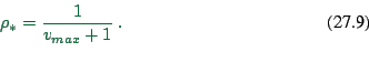
It turns out that, after transients have died out, there are two regimes (Figs. 27.4 and 27.5):
 |
(27.8) |
 |
(27.9) |
![\includegraphics[width=0.6\textwidth]{184tty-fig.eps}](img364.png)
|
Stochastic traffic CA (STCA)
One can add noise to the CA model by adding a randomization term:
Real traffic may have a strong hysteresis effect near maximum flow;
there is however no agreement among researchers if or under which
circumstances this effect truly exists. If it exists, it looks as
follows: When coming from low densities, traffic stays laminar and at
free speed up to a certain density ![]() (see
Fig. 27.7). Above that, traffic ``breaks down''
into start-stop traffic. When lowering the density again, however, it
does not become laminar again until
(see
Fig. 27.7). Above that, traffic ``breaks down''
into start-stop traffic. When lowering the density again, however, it
does not become laminar again until ![]() , which is
significantly smaller than
, which is
significantly smaller than ![]() , up to 30%
(63,64). This effect can be
included into the above rules by making acceleration out of stopped
traffic weaker than acceleration at all other speeds, for example
by:
, up to 30%
(63,64). This effect can be
included into the above rules by making acceleration out of stopped
traffic weaker than acceleration at all other speeds, for example
by:
 |
A modification to make the STCA more realistic is the so-called time-oriented CA (TOCA) (19). The motivation is to introduce a higher amount of elasticity in the car following, that is, vehicles should accelerate and decelerate at larger distances to the vehicle ahead than in the STCA, and resort to emergency braking only if they get too close. For the TOCA velocity update, the following operations need to be done in sequence for each car:
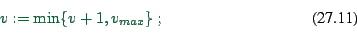 |
(27.11) |
 |
(27.12) |
Dependence on the velocity of the car ahead
It makes sense to assume that velocity difference between vehicles should be included. The idea is that if the car ahead is faster, then this adds to one's effective gap and one may drive faster than without this. In the CA context, the challenge is to retain a collision-free parallel update. Wolf (127) achieves this by going through the velocity update twice, where in the second round any major velocity changes of the vehicle ahead are included. Barrett et al. (11) instead additionally look at the gap of the vehicle ahead. The idea here is that, if we know the gap of the vehicle ahead, and we make assumptions about the driver behavior of the vehicle ahead, then we can compute bounds on the behavior of the vehicle ahead in the next time step.
Theory
CA rules can also be analyzed analytically, by means of statistical techniques which look at sequences of configurations of the dynamical evolution of the system (e.g. 106,30,105). Note that this is possible because the cellular approach makes the dynamical states countable: There is only a finite number of possible states for a given number of cells.
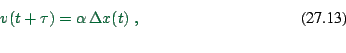
Making both space and time continuous results in coupled differential
equations. Such models for car following were established quite some
time ago (e.g. 48, and references therein). Most of them
also use in one way or other the reaction time argument of
Sec. 27.4.1 (as they should).
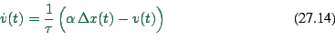
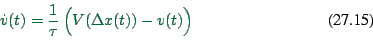
For example, one could use
One can
expand
![]() ,
drop
second order terms, and rearrange, resulting in
,
drop
second order terms, and rearrange, resulting in
A generalization of Eq. (27.14) is to replace
![]() with a function
with a function
![]() :
:
[[bando ref]]
The ``classic'' car-following model family
(48) comes from taking a time-derivative of the
reaction-time relation Eq. (27.13), leading to
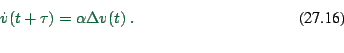 |
(27.16) |
For computer implementations, models with continuous time are inconvenient, since time needs to be discretized in one way or other. Because of the reaction delay, many of these car-following equations are delay equations, where considerable effort needs to be spent for faithful numerical results. Given this observation, it seems to be simpler to build models that use discretized time to their advantage (see next section). This is not to say that continuous car-following models are useless; indeed, they continue to contribute to our understanding of the matter (e.g. 6,5). We would expect, however (see below), that any faithful discretization of these equations will run a lot more slowly on a computer than the model presented in the next section, which explicitly uses discrete time.
Another possible implementation of continuous space and time would be event-driven. This works best when particles move with constant velocity for periods of time, interrupted by events where they change it. Molecular dynamics with hard core interactions is an example. Since human driving behavior can probably indeed be characterized like that (125), this should be a promising approach. However, parallel implementations of event-driven simulations are hard and therefore large scale simulations currently not done with this method.
A disadvantage of the CA approach to traffic is that the coarse-gained description makes fine tuning of many properties difficult. For example, it is difficult to represent fine-grained differences in speed limits, or different acceleration profiles.
On the other hand, the use of coupled ordinary differential equations
turns out to be inconvenient for traffic simulations, in particular
because of the explizit handling of the reaction time, which means
that for numerical integration one needs to maintain the entire
dynamical history between ![]() and
and ![]() in increments of the time
discretization
in increments of the time
discretization ![]() . There are however also models that are
continuous in space but coarse-grained discrete in time which work
extremely well for traffic
(49,104,131,68,66).
The reason for this
is that drivers have a reaction delay of about one second, and it is
advantageous to use this reaction delay as the time step for the
micro-simulation. From a practical point of view, traffic models
which use discrete time but continuous space are numerically as
efficient as the CA models but are much easier to calibrate.
Obviously, a multitude of models is possible here - as is with CAs.
We want to concentrate on a single model, a model described by
Krauß (68,66). This model is
particularly well understood.
. There are however also models that are
continuous in space but coarse-grained discrete in time which work
extremely well for traffic
(49,104,131,68,66).
The reason for this
is that drivers have a reaction delay of about one second, and it is
advantageous to use this reaction delay as the time step for the
micro-simulation. From a practical point of view, traffic models
which use discrete time but continuous space are numerically as
efficient as the CA models but are much easier to calibrate.
Obviously, a multitude of models is possible here - as is with CAs.
We want to concentrate on a single model, a model described by
Krauß (68,66). This model is
particularly well understood.
The approach starts again from the reaction time argument
(Sec. 27.4.1), this time taking into account the possibility
that the two cars can have different velocities. This results in the
condition that one's braking distance plus the distance that one
drives until one reacts should be smaller than the braking distance of
the car ahead plus the space in between the two vehicles. Formally,
this yields
This can be used to derive (see Fig. 27.8) a simple update
scheme for the dynamical state of a car:
The terms can be interpreted as follows:
 |
(27.23) |
 |
(27.24) |
Note that for ![]() and
and ![]() we recover the STCA rule.
we recover the STCA rule.
Note that this is the same as the CA rule.
Again, this is the same as the CA rule.
![\includegraphics[width=0.6\hsize]{fdiag-184-fig.eps}](img365.png)
![\includegraphics[width=0.6\hsize]{fdiag-184-s2s-fig.eps}](img377.png)
![\begin{displaymath}
\dot{v}(t+\tau) = \alpha \, \frac{[v(t+\tau)]^l}{ [\Delta x(t)]^m } \,
\Delta v(t) \ .
\end{displaymath}](img395.png)