The intuition for kinematic waves is easy to understand. Start with five vehicles of velocity zero in five adjoining cells. In the first time step, only the first vehicle can move. In the second time step, the second vehicle can start, etc. However, in the meantime it can happen that another vehicle joins the queue at the tail.
Given the right conditions (more vehicles joining at the tail than leaving at the head), this results in a cluster of vehicles of velocity zero and that cluster will move against the traffic direction. Note that the vehicle composition of this cluster is constantly changing - from the perspective of a driver, you join the jam from the end, the jam ``moves through you'', and then you can start again (look at the two trajectories in the lower part of Fig. 27.4 for an illustration). This is a standard wave phenomenon.
A detailed introduction into such waves can for example be found by Haberman (52). Here, we will just [[word?]] give an overview for people who have some prior knowledge about partial differential wave equations.
One way to see all the connections [[word?]] is to start from the
standard equation of continuity, which needs to be fulfilled as long
as our traffic obeys mass conservation (no vehicles leaving or
joining). This equation is
![]() (equation of continuity). This equation can be easily
understood when it is discretized (with discretization constants
(equation of continuity). This equation can be easily
understood when it is discretized (with discretization constants
![]() and
and ![]() ):
):
We now need a relation between ![]() and
and ![]() . Let us assume that
. Let us assume that ![]() is a function of
is a function of ![]() only, i.e. the total differential is
only, i.e. the total differential is
![]() . The meaning of this (instantaneous
velocity adaptation) will be discussed below. The resulting theory is
also called the Lighthill-Whitham-Richards (LWR) theory
(70). [[Richards ref]] The equation of continuity can
immediately re-written as
. The meaning of this (instantaneous
velocity adaptation) will be discussed below. The resulting theory is
also called the Lighthill-Whitham-Richards (LWR) theory
(70). [[Richards ref]] The equation of continuity can
immediately re-written as
![]() (LWR equation), where
(LWR equation), where ![]() is some externally
given but as of yet unspecified function.
is some externally
given but as of yet unspecified function.
Since we now have a fully defined partial differential equation, we
can try to understand some of it. A typical first step is
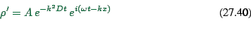
``linearization''. For this, ![]() is replaced by
is replaced by
![]() , with
, with
![]() (stationary) and
(stationary) and
![]() (homogeneous); this is always
possible. One now assumes that
(homogeneous); this is always
possible. One now assumes that ![]() is small. Functions in
is small. Functions in
![]() are Taylor-expanded:
are Taylor-expanded:
 |
(27.26) |
 |
(27.27) |
 |
(27.30) |
Linearization is not very useful for traffic, since it assumes small
![]() , which is often not fulfilled in traffic. Let us thus look at
a macroscopic front with speed
, which is often not fulfilled in traffic. Let us thus look at
a macroscopic front with speed ![]() . Let us go to the same reference
system as the front. In that reference system, the flow to the left
of the front needs to be the same as the flow to the right of the
front, because otherwise there would either be an excess or a lack of
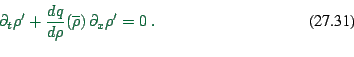
``material'' at the front. Let us denote variables in the reference
system of the front with a tilde. In equations, the statement means
. Let us go to the same reference
system as the front. In that reference system, the flow to the left
of the front needs to be the same as the flow to the right of the
front, because otherwise there would either be an excess or a lack of
``material'' at the front. Let us denote variables in the reference
system of the front with a tilde. In equations, the statement means
 |
(27.31) |
We can now analyse our deterministic CA (Sec. 27.4.2) in terms of kinematic waves (see also Fig. 27.5):
 |
(27.32) |
[[might be good to do xfig here too]]
The inflow is somewhere on the ``laminar'' branch of the fundamental
diagram. That means that the slope of the line connecting to
![]() is either
is either ![]() or less steep. The inflow front thus
moves backwards with speed
or less steep. The inflow front thus
moves backwards with speed ![]() or less -- that is, the jam will
eventually vanish except when inflow is exactly equal to maximum flow.
or less -- that is, the jam will
eventually vanish except when inflow is exactly equal to maximum flow.
One can treat queues at traffic lights similarly. While the traffic
light is red, ![]() and thus the outflow front does not move
(which we know since the first car is waiting at the red light). The
inflow front moves backwards with
and thus the outflow front does not move
(which we know since the first car is waiting at the red light). The
inflow front moves backwards with
![]() .
.
Once the traffic light turns green, the outflow front now moves
backwards with ![]() , while the inflow front keeps moving backwards
with
, while the inflow front keeps moving backwards
with ![]() . The situation remains like that until the outflow
front catches up with the inflow front. And if the traffic light
turns red before that, one needs to include that effect
(Fig. 27.12).
. The situation remains like that until the outflow
front catches up with the inflow front. And if the traffic light
turns red before that, one needs to include that effect
(Fig. 27.12).
The kinematic theory is entirely sufficient to understand the most important theoretical aspects of traffic flow. This section goes a little bit beyond that, by providing an outlook what else could be done.
The STCA and in particular the slow-to-start model are not entirely described by the kinematic theory. This is in part due to the stochastic elements, which are not captured in the equation. It is also due to the hysteresis which is displayed by the slow-to-start model (Fig. 27.7) but not by kinematic theory. This motivates to look for fluid-dynamical equations for traffic that capture effects beyond the kinematic theory. Two extensions of the kinematic theory will be discussed.
Addition of diffusive terms
Diffusive terms can be justified for many reasons. The result is an
equation like
 |
(27.33) |
 |
(27.34) |
Addition of inertia
Above, we have assumed that flow ![]() is a function of the density
is a function of the density
![]() only. This is in general not true -- if a driver suddenly
comes into denser traffic, she/he will need some time to adjust; the
same is true if density suddenly decreases. That means that velocity
will be delayed in its adaptation to density.
only. This is in general not true -- if a driver suddenly
comes into denser traffic, she/he will need some time to adjust; the
same is true if density suddenly decreases. That means that velocity
will be delayed in its adaptation to density.
A way to capture this is to add an equation for the velocity. One can
for example use the car following equation (27.15)
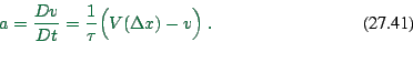 |
(27.35) |
The translation of the particle-oriented ![]() into the
fluid-dynamical
into the
fluid-dynamical
![]() yields
yields
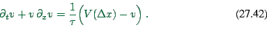 |
(27.36) |
We need however ![]() instead of
instead of ![]() , and we also need
, and we also need
![]() measured at the location of the vehicle and not in the middle
between two vehicles, where
measured at the location of the vehicle and not in the middle
between two vehicles, where ![]() is
measured.27.7This is the mathematical reason for what is usually called the
anticipation term
is
measured.27.7This is the mathematical reason for what is usually called the
anticipation term
 |
(27.39) |
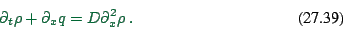
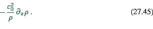
In addition, we will again add a diffusion term,
![]() . Overall, one obtains the momentum equation
. Overall, one obtains the momentum equation
![]() Note that we still need to specify
Note that we still need to specify
![]() , which is the same information as
, which is the same information as ![]() introduced after
Eq. (27.25). The only difference is that we now allow that it can take some
time until velocities have adjusted accordingly. Indeed, the
relaxation time is
introduced after
Eq. (27.25). The only difference is that we now allow that it can take some
time until velocities have adjusted accordingly. Indeed, the
relaxation time is ![]() . If we let
. If we let ![]() go to zero, then the
momentum equations becomes
go to zero, then the
momentum equations becomes ![]() , which means instantaneous
adaptation.
, which means instantaneous
adaptation.
There is quite a lot of theory about this equation and its meaning for traffic (e.g. 61,53). Much of the behavior of the micro-simulation models can be explained using these equations; in fact, much of it was first observed in the fluid-dynamical equations. This, however, would be a full class in traffic flow theory and would thus go beyond the scope of this text.
[[breakdown and recovery. do I really want that for this text?]]
![\includegraphics[width=0.8\hsize]{cell-trans-fig.eps}](img437.png)
![\includegraphics[width=0.47\hsize]{tangent-fig.eps}](img462.png)
![\includegraphics[width=0.53\hsize]{tangent-back-fig.eps}](img463.png)
![\includegraphics[width=0.5\textwidth]{secant-fig.eps}](img471.png)
![\includegraphics[width=0.6\hsize]{tr-light-fig.eps}](img487.png)