- ... problem.4.1
- In C,
this would be done via malloc.
.
.
.
.
.
.
.
.
.
.
.
.
.
.
.
.
.
.
.
.
.
.
.
.
.
.
.
.
.
.
- ...
here.4.2
- For experts: The main reason why we do not use it is because
constructors are not inherited. For templatized classes, as will be
useful for the network construction (Sec. 10), this
means that each change of the constructor arguments in the template
methods necessitates corresponding changes in all derived classes. We
found that rather inconvenient.
.
.
.
.
.
.
.
.
.
.
.
.
.
.
.
.
.
.
.
.
.
.
.
.
.
.
.
.
.
.
- ...
etc.:7.1
- Again, there are specific commands in the STL to achieve the same
thing. We leave that to the experts.
.
.
.
.
.
.
.
.
.
.
.
.
.
.
.
.
.
.
.
.
.
.
.
.
.
.
.
.
.
.
- ...
vector.7.2
- One could use allocate, but the use of push_back
preserves at least somewhat the look and feel of a traditional array.
.
.
.
.
.
.
.
.
.
.
.
.
.
.
.
.
.
.
.
.
.
.
.
.
.
.
.
.
.
.
- ... skipped.9.1
- If this token is not
zero, then the following numbers are not only NodeIDs, but also
passenger IDs. We do not want to treat this case.
.
.
.
.
.
.
.
.
.
.
.
.
.
.
.
.
.
.
.
.
.
.
.
.
.
.
.
.
.
.
- ... obtained.12.1
- Earlier versions, by Transims and also by ourselves, aggregated the
event information into the time bins either directly in the traffic
simulation, or by some external module, and wrote the result into a
file. The typical information given in that file was a time, say
``900 sec'', and a corresponding link travel time. In
implementations, there was then always confusion if this referred to a
time bin going from 1 to 900, or to a time bin going from 900 to 1799.
The intention was the first, but unfortunately time%900 (where
% is the modulo function) puts 0 to 899 into one time bin and
900 to 1799 into another one, resulting in many errors. Clearly, this
is a trivial problem, but one that continuously caused problems.
.
.
.
.
.
.
.
.
.
.
.
.
.
.
.
.
.
.
.
.
.
.
.
.
.
.
.
.
.
.
- ... them.13.1
- This is truly awkward. In our research, we put the new plans into a
data base, which keeps track of all plans. Then we dump out
the plans we want. That solution is much cleaner, but besides being
more difficult to implement, it is also slow, so it is not the final
answer.
.
.
.
.
.
.
.
.
.
.
.
.
.
.
.
.
.
.
.
.
.
.
.
.
.
.
.
.
.
.
- ... 100.14.1
- We are looking for the departure time distribution of the whole
population, not just of the replanned population. This is best
retrieved from the events file.
.
.
.
.
.
.
.
.
.
.
.
.
.
.
.
.
.
.
.
.
.
.
.
.
.
.
.
.
.
.
- ... priority.18.1
- Note that the winning links are not the ones that come first, but the
ones that come first after the outgoing link was treated. For
example, assume a configuration where links 1 and 3 are incoming into
link 2, and assume that they are processed in sequence 1, 2, 3.
[[fig?]] Also assume that under congested conditions initially all
links are completely full. Then link 1 is processed first, but link 2
is full, so no vehicle can move. Then link 2 is processed, and some
vehicles move out, opening up some space. Finally, link 3 is
processed, and since there is some space on link 2, some vehicles can
move.
.
.
.
.
.
.
.
.
.
.
.
.
.
.
.
.
.
.
.
.
.
.
.
.
.
.
.
.
.
.
- ... iteration.19.1
- To be entirely precise, one would have to say that the route is best
based on the time-averaged information that the router uses.
.
.
.
.
.
.
.
.
.
.
.
.
.
.
.
.
.
.
.
.
.
.
.
.
.
.
.
.
.
.
- ...fig:parallel):25.1
- Instead of ``split links'', the terms ``boundary links'', ``shared
links'', or ``distributed links'' are sometimes used. As is well
known, some people use ``edge'' instead of ``link''.
.
.
.
.
.
.
.
.
.
.
.
.
.
.
.
.
.
.
.
.
.
.
.
.
.
.
.
.
.
.
- ... CPUs.25.2
- For simplicity, we do not differentiate between CPUs and
computational nodes. Computational nodes can have more than one CPU
-- an example is a network of coupled PCs where each PC has Dual
CPUs.
.
.
.
.
.
.
.
.
.
.
.
.
.
.
.
.
.
.
.
.
.
.
.
.
.
.
.
.
.
.
- ... Mbit/s.25.3
- Our measurements have consistently shown that node bandwidths are
lower than network bandwidths. Even CISCO itself specifies
148000 packets/sec, which translates to about 75 Mbit/sec, for the
100 Mbit switch that we use.
.
.
.
.
.
.
.
.
.
.
.
.
.
.
.
.
.
.
.
.
.
.
.
.
.
.
.
.
.
.
- ... small.25.4
- An event-driven simulation could be a counter-example: Depending on
the implementation, it could be extremely fast on a single CPU up to
medium problem sizes, but slow on a parallel machine.
.
.
.
.
.
.
.
.
.
.
.
.
.
.
.
.
.
.
.
.
.
.
.
.
.
.
.
.
.
.
- ... CPUs.25.5
- This is possible because of the specific purpose Transims is
designed for. In real time applications, where absolute speed
between request and response matters, the situation is
different (27).
.
.
.
.
.
.
.
.
.
.
.
.
.
.
.
.
.
.
.
.
.
.
.
.
.
.
.
.
.
.
- ....27.1
- From a theoretical perspective, it is questionable if this averaging
is a good idea. It is however necessary to compare with field data.
.
.
.
.
.
.
.
.
.
.
.
.
.
.
.
.
.
.
.
.
.
.
.
.
.
.
.
.
.
.
- ... complicated.27.2
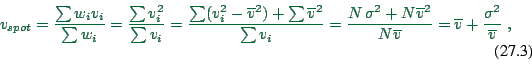
- Assume that
 is a sequence of speed measurements of different
vehicles for the space-mean speed. The probability of a vehicle of
veloctiy
is a sequence of speed measurements of different
vehicles for the space-mean speed. The probability of a vehicle of
veloctiy  to cross a sensor within a given time period is
proportional to .
Thus,
in order to obtain spot speed from
, each has to be weighted by
to cross a sensor within a given time period is
proportional to .
Thus,
in order to obtain spot speed from
, each has to be weighted by  :
:
 |
(27.3) |
where  is the variance of the velocity measurement.
This
confirms that spot speed is larger than space-mean speed, and the
difference increases with increasing velocity fluctuations.
-
An alternative derivation is, for example,
in (48).
is the variance of the velocity measurement.
This
confirms that spot speed is larger than space-mean speed, and the
difference increases with increasing velocity fluctuations.
-
An alternative derivation is, for example,
in (48).
.
.
.
.
.
.
.
.
.
.
.
.
.
.
.
.
.
.
.
.
.
.
.
.
.
.
.
.
.
.
- ... used.27.3
- ``Gap'' denotes the space from my front bumper to the rear bumper of
the car ahead, sometimes minus some safety space one would like to
have. Space headway is used less uniformly; for example, it sometimes
denotes the front-bumper-to-front-bumper space, thus including the
length of the car ahead.
.
.
.
.
.
.
.
.
.
.
.
.
.
.
.
.
.
.
.
.
.
.
.
.
.
.
.
.
.
.
- ... ahead.27.4
- Car-following models have a tendency to not distinguish cleanly
between
 (which is space between cars) and
  (which is
usually front-bumper-to-front-bumper distance). As long as vehicles
do not pass each other, these differences are indeed irrelevant.
(which is
usually front-bumper-to-front-bumper distance). As long as vehicles
do not pass each other, these differences are indeed irrelevant.
.
.
.
.
.
.
.
.
.
.
.
.
.
.
.
.
.
.
.
.
.
.
.
.
.
.
.
.
.
.
- ...27.5
- Note that this formulation includes the effect of different
velocities, but it assumes that acceleration of the follower is
zero ().
.
.
.
.
.
.
.
.
.
.
.
.
.
.
.
.
.
.
.
.
.
.
.
.
.
.
.
.
.
.
- ... minutes.27.6
- There are several elements:
.
.
.
.
.
.
.
.
.
.
.
.
.
.
.
.
.
.
.
.
.
.
.
.
.
.
.
.
.
.
- ...
measured.27.7
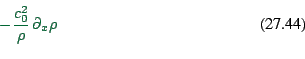
- Linearization yields
 |
(27.37) |
The second term (``anticipation term'') is usually approximated by
 |
(27.38) |
in analogy to the sound wave solution of the Navier-Stokes equations.
[[fig for this?]]
.
.
.
.
.
.
.
.
.
.
.
.
.
.
.
.
.
.
.
.
.
.
.
.
.
.
.
.
.
.
- ....28.1
- Conventionally, one uses
 here; I will use
  because that's
what we have used in traffic flow theory.
because that's
what we have used in traffic flow theory.
.
.
.
.
.
.
.
.
.
.
.
.
.
.
.
.
.
.
.
.
.
.
.
.
.
.
.
.
.
.
- ... slow.28.2
- The intuitive reason both for convergence and for slowness is that
 always diverges, no matter what
  is. This
means that any initial contributions to
is. This
means that any initial contributions to  can always be fully
corrected by later iterations. However, it is also clear that such
late corrections take very many iteration steps.
can always be fully
corrected by later iterations. However, it is also clear that such
late corrections take very many iteration steps.
.
.
.
.
.
.
.
.
.
.
.
.
.
.
.
.
.
.
.
.
.
.
.
.
.
.
.
.
.
.
- ... learn).31.1
- More precisely: The agent cannot assume that the probabilities are
constant since the other agents also learn. However, in the long run
all probabilities will become constant.
.
.
.
.
.
.
.
.
.
.
.
.
.
.
.
.
.
.
.
.
.
.
.
.
.
.
.
.
.
.
- ...
data.32.1
- Bluntly, one can always fit a straight line to a data
cloud.
.
.
.
.
.
.
.
.
.
.
.
.
.
.
.
.
.
.
.
.
.
.
.
.
.
.
.
.
.
.
- ... set.32.2
- Note, though, that it is certainly
desirable to have reasonable microscopic rules.
.
.
.
.
.
.
.
.
.
.
.
.
.
.
.
.
.
.
.
.
.
.
.
.
.
.
.
.
.
.
- ...
 32.3
32.3
- If this rule would ask for a negative velocity, then $v=0$ is chosen.
.
.
.
.
.
.
.
.
.
.
.
.
.
.
.
.
.
.
.
.
.
.
.
.
.
.
.
.
.
.
- ...)32.4
- Weights are used because of extensibility towards ``lane changing for
plan following''. See below.
.
.
.
.
.
.
.
.
.
.
.
.
.
.
.
.
.
.
.
.
.
.
.
.
.
.
.
.
.
.
- ... change32.5
- In the current version, the lane change is actually still rejected
with a probability of 0.01 even when all the rules are fulfilled.
This is in order to break the following artifact or variations of it:
Assume one lane is completely occupied and one is completely empty.
The above rule set will result in these vehicles just changing back
and forth between the lanes--the vehicles will never get smeared out
across the lanes. See Ref. (101) for
more details.
.
.
.
.
.
.
.
.
.
.
.
.
.
.
.
.
.
.
.
.
.
.
.
.
.
.
.
.
.
.
- ... situation.32.6
- In a deeper sense, the problem is caused by the fact that the
underlying decision making dynamics has a time scale which is smaller
than the time resolution of the simulation. The simulation thus must
resolve the conflict by other means (8).
.
.
.
.
.
.
.
.
.
.
.
.
.
.
.
.
.
.
.
.
.
.
.
.
.
.
.
.
.
.
- ...
link.32.7
- Vehicles may accelerate or slow down before they actually reach the
intersection. See below.
.
.
.
.
.
.
.
.
.
.
.
.
.
.
.
.
.
.
.
.
.
.
.
.
.
.
.
.
.
.
- ... them.32.8
- Again, technically the vehicles only reserve cells on the destination
links. The actual move through the intersection happens later and can
also be postponed if after the velocity update the vehicle actually
does not make it to the intersection.
.
.
.
.
.
.
.
.
.
.
.
.
.
.
.
.
.
.
.
.
.
.
.
.
.
.
.
.
.
.
- ...
vehicle,32.9
- I.e. there is a probability of
 that the vehicle will
not accelerate in the given time step.
that the vehicle will
not accelerate in the given time step.
.
.
.
.
.
.
.
.
.
.
.
.
.
.
.
.
.
.
.
.
.
.
.
.
.
.
.
.
.
.
- ... conditions.32.10
- Note that the situation slightly different when the speed of the
vehicle on the major link is zero - see below.
.
.
.
.
.
.
.
.
.
.
.
.
.
.
.
.
.
.
.
.
.
.
.
.
.
.
.
.
.
.
- ...
simulations.32.11
- Route plans are simply necessary to be consistent with the way the
simulation is normally used; for the test cases we use very few types
of generic route plans (like ``enter the microsimulation and keep on
driving in a circle indefinitely'') and replicate them with different
starting times to fulfill our needs. This is not much different from
departure rates.
.
.
.
.
.
.
.
.
.
.
.
.
.
.
.
.
.
.
.
.
.
.
.
.
.
.
.
.
.
.
- ... m.32.12
- The ``magical'' number of
 sites is equal to the maximum velocity
of
sites is equal to the maximum velocity
of  sites/update. This ensures that each vehicle is
counted at least once.
sites/update. This ensures that each vehicle is
counted at least once.
.
.
.
.
.
.
.
.
.
.
.
.
.
.
.
.
.
.
.
.
.
.
.
.
.
.
.
.
.
.
- ... discrepancies.32.13
- This explains the differences to the TRB
preprint version of this paper, which contained results from the
experimental code.
.
.
.
.
.
.
.
.
.
.
.
.
.
.
.
.
.
.
.
.
.
.
.
.
.
.
.
.
.
.
- ... times.36.1
- Since the whole travel of each traveller in our simulation consists
of exactly one trip, ``trip time'' and ``travel time'' will be used
synonymously.
.
.
.
.
.
.
.
.
.
.
.
.
.
.
.
.
.
.
.
.
.
.
.
.
.
.
.
.
.
.
- ....36.2
- In contrast to the routing module, no time-dependence was used
here although future implementations should do so.
.
.
.
.
.
.
.
.
.
.
.
.
.
.
.
.
.
.
.
.
.
.
.
.
.
.
.
.
.
.
- ... area.36.3
- This really depends on the cost function which is used. Most cost
functions set link speed
 to a very low number (but not to zero)
at high volumes. Since link costs are proportional to
to a very low number (but not to zero)
at high volumes. Since link costs are proportional to  , where
 link length, one has that congested links do not contribute much
to the cost of a route as long as these links are short and rare.
In consequence, much too high volumes can be assigned to such links.
link length, one has that congested links do not contribute much
to the cost of a route as long as these links are short and rare.
In consequence, much too high volumes can be assigned to such links.
.
.
.
.
.
.
.
.
.
.
.
.
.
.
.
.
.
.
.
.
.
.
.
.
.
.
.
.
.
.
- ...
31\%.36.4
- This number is larger than one would expect from
Fig. 36.5. The reason is that many high volume streets
were not counted in both years, thus leading to a smaller mean, which
leads to a larger relative error.
.
.
.
.
.
.
.
.
.
.
.
.
.
.
.
.
.
.
.
.
.
.
.
.
.
.
.
.
.
.
- ... close.36.5
- For certain -much simpler- systems, one can show that many plausible
iteration schemes converge towards the same state (Hofbauer and
Sigmund, 1998).
.
.
.
.
.
.
.
.
.
.
.
.
.
.
.
.
.
.
.
.
.
.
.
.
.
.
.
.
.
.
 essentially means an
equation of type
essentially means an
equation of type
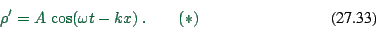
 ) is a wave equation. As one can easily verify, it has
wave length
) is a wave equation. As one can easily verify, it has
wave length  , that is, the function is periodic under
additions of
, that is, the function is periodic under
additions of  is called the wave number.
Similarly, the function is periodic under additions of
is called the wave number.
Similarly, the function is periodic under additions of  to
to  ;
;  is called the frequency.
 . In Eq.
  , at time
  there is a wave
crest at position
there is a wave
crest at position  . At time
  , which means a velocity
 .
.