First, the field count data is compared with the results of our simulation runs directly for every link. For comparison, the results of the ``EMME/2 study'' are also shown. Fig. 36.4 shows the typical scatterplots, with field data on the x-axis and simulation results for the same links on the y-axis. Note that both axes are logarithmic.
The first observation is that the plots look remarkably similar in structure. All three studies give relatively unbiased results for high flows, and underestimate low volumes. In addition, there are a few data points where simulation and reality are rather far apart.
At closer inspection, one notes that EMME/2 is somewhat overestimating high volumes, whereas our simulations are underestimating them. This is confirmed by bias calculations (see below). Such an effect is consistent with what one would expect: The Portland Metro assignment model for the presented results does not have a flow cutoff at capacity, so that it is possible to actually put more flow on a link than that link has capacity. This happens in particular at bottlenecks on short links in an otherwise relatively uncongested area.36.3 The queue model traffic simulation tends to behave in the opposite way. If demand is higher than capacity, the queue spills back. Once this queue reaches another intersection, that intersection will normally be blocked for all directions, not just for the direction into the congested link. This is a consequence of the fact that the queue model neglects multi-lane effects at intersections. This means, for instance, that a car waiting for a chance to make a left turn blocks all following cars on this link. This tends to cause unrealistically large spill backs.
When one compares sim-80 to sim-100, the flows for sim-80 are closer to the field data for high volumes, and farther away for medium volumes. It is striking that demand reduction by as much as 20% changes the resulting flows so little. This adds to the conjecture that measured flows in a network depend as much on the network structure as on the demand structure.
For more detailed information, one can look at links in different
classes regarding field data and direction (Table 36.1). For
each class ![]() we calculated the mean absolute and relative bias, i.e.
we calculated the mean absolute and relative bias, i.e.
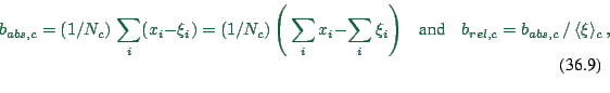 |
(36.9) |
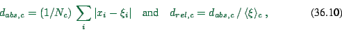 |
(36.10) |
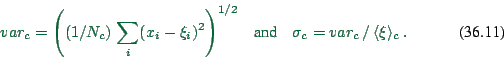 |
(36.11) |
Links were classified by visual inspection into links leading towards the Portland downtown area, and all other links. The tables show that our simulations are underestimating the flows on the ``other'' links more than they are underestimating the flows on the links towards downtown. Visual inspection of the simulations reveals that this is probably a result of too much demand (and thus congestion) for traffic away from the downtown area. This is what one would expect from our simplifications: We are assuming a spatially homogeneous trip time distribution; yet, one would expect that people who live downtown moved there because they have a higher dislike of long trip times than the average population.
Regarding the size classes, sim-100 systematically
underestimates volumes except for class 1 (![]() ). Sim-80
underestimates less for class 6 (
). Sim-80
underestimates less for class 6 (![]() ), underestimates more for all
intermediate classes, and is nearly unbiased for class 1. The
interpretation of this is that in sim-100, traffic on the major roads
is so congested that the routes are pushed onto the smaller streets.
The EMME/2 studies, in contrast, systematically over-estimate volumes.
Similar to our results, the ratio of traffic on small vs traffic on
large roads is too high. Quite possibly, the fastest path search that
is used in both approaches makes simulated travelers accept
complicated detours on minor streets more easily than in the real
world.
), underestimates more for all
intermediate classes, and is nearly unbiased for class 1. The
interpretation of this is that in sim-100, traffic on the major roads
is so congested that the routes are pushed onto the smaller streets.
The EMME/2 studies, in contrast, systematically over-estimate volumes.
Similar to our results, the ratio of traffic on small vs traffic on
large roads is too high. Quite possibly, the fastest path search that
is used in both approaches makes simulated travelers accept
complicated detours on minor streets more easily than in the real
world.
Last, one should also remember that the estimated error of the field
counts is assumed to be no better than ![]() . We will come
back to this point in the discussion.
. We will come
back to this point in the discussion.
In summary, one can say the following: Our simulations are far enough progressed to allow tentative comparisons to real world volume counts. The simulations done for this investigation lead to traffic flows with volumes that are somewhat low when compared to reality. Due to the complexity of the approach, there can be many reasons for this, and the systematic analysis of these effects should be the subject of future research.
![\includegraphics[width=0.45\textwidth]{scatter-100-gpl.eps}](img916.png)
![\includegraphics[width=0.45\textwidth]{scatter-080-gpl.eps}](img917.png)
![\includegraphics[width=0.45\textwidth]{scatter-e2-gpl.eps}](img918.png)
|
|
|