The approach that is maybe closest to our work are the discrete choice
models (Ben-Akiva and Lerman, 1985). As is
well known, in that approach the utility ![]() of an alternative
of an alternative ![]() is assumed to have a systematic component
is assumed to have a systematic component ![]() and a random component
and a random component
![]() . Under certain assumptions for the random component this
implies that the probability
. Under certain assumptions for the random component this
implies that the probability ![]() (called choice function) to select
alternative
(called choice function) to select
alternative ![]() is
is
In this paper, the ``psychological'' function ![]() is obtained
from ``observed'' trip time distributions, using new methods of
micro-simulating large geographical regions. The core idea is that an
observed trip time distribution
is obtained
from ``observed'' trip time distributions, using new methods of
micro-simulating large geographical regions. The core idea is that an
observed trip time distribution ![]() can be decomposed into an
accessibility part
can be decomposed into an
accessibility part ![]() and an acceptance (
and an acceptance (![]() choice) function
choice) function
![]()
Given a micro-simulation of traffic, ![]() can be derived from
the simulation result. For a given home location (and a given assumed
starting time), one can build a tree of time-dependent shortest paths,
and every time one encounters a workplace at time-diestance
can be derived from
the simulation result. For a given home location (and a given assumed
starting time), one can build a tree of time-dependent shortest paths,
and every time one encounters a workplace at time-diestance ![]() , one
adds that to the count for trip time
, one
adds that to the count for trip time ![]() . The challenge is that this
result depends on the traffic: Given the same geographic
distribution of workplaces, these are farther away in terms of trip
time when the network is congested than when it is empty. That is,
given the function
. The challenge is that this
result depends on the traffic: Given the same geographic
distribution of workplaces, these are farther away in terms of trip
time when the network is congested than when it is empty. That is,
given the function ![]() , one can obtain the function
, one can obtain the function
![]() via micro-simulation, i.e.
via micro-simulation, i.e.
![]() , where
, where ![]() is the micro-simulation which can be seen
as a functional operating on the whole function
is the micro-simulation which can be seen
as a functional operating on the whole function ![]() . The
problem then is to find the macroscopic (i.e., averaged over all
trips) function
. The
problem then is to find the macroscopic (i.e., averaged over all
trips) function ![]() self-consistently such that, for all
travel times
self-consistently such that, for all
travel times ![]() ,
,
For this, a relaxation technique is used. It starts with a guess for
![]() and from there generates
and from there generates
![]() via
simulation. A new guess for
via
simulation. A new guess for ![]() is then obtained via
is then obtained via
Real census data is used for ![]() (see ``census-100''-curve in
Fig. 36.3; from now on denoted as
(see ``census-100''-curve in
Fig. 36.3; from now on denoted as ![]() ).
People usually give their trip times in minute-bins as the highest
resolution. Since our simulation is driven by one-second time steps we
need to smooth the data in order to get a continuous function instead
of the minute-histogram. Many possibilities for smoothing exist; one
of them is the beta-distribution approach in Wagner and Nagel (1999).
Here, we encountered problems with that
particular fit for small trip times: Since that fit grows out of zero
very quickly, the division
).
People usually give their trip times in minute-bins as the highest
resolution. Since our simulation is driven by one-second time steps we
need to smooth the data in order to get a continuous function instead
of the minute-histogram. Many possibilities for smoothing exist; one
of them is the beta-distribution approach in Wagner and Nagel (1999).
Here, we encountered problems with that
particular fit for small trip times: Since that fit grows out of zero
very quickly, the division
![]() had a tendency to result
in unrealistically large values for very small trip times. We
therefore used a piecewise linear fit with the following properties:
(i) For trip time zero, it starts at zero. (ii) At trip times
2.5 min, 7.5 min, 12.5 min, etc. every five minutes, the area under
the fitted function corresponds to the number of trips shorter than
this time according to the census data.
had a tendency to result
in unrealistically large values for very small trip times. We
therefore used a piecewise linear fit with the following properties:
(i) For trip time zero, it starts at zero. (ii) At trip times
2.5 min, 7.5 min, 12.5 min, etc. every five minutes, the area under
the fitted function corresponds to the number of trips shorter than
this time according to the census data.
Obtaining ![]() itself via simulation is by no means trivial.
It is now possible to micro-simulate large metropolitan regions in
faster than real time, where ``micro''-simulation means that each
traveler is represented individually. The model used here is a simple
queuing type traffic flow model described in Simon and Nagel (1999).
However, even if one knows the origins
(home locations) and destinations (workplaces), one still needs to
find the routes that each individual takes. This ``route assignment''
is typically done via another iterative relaxation, where, with
location choice fixed, each individual attempts to find faster routes
to work. Rickert (1998) and Nagel and Barrett (1997)
give more detailed
information about the route-relaxation procedure; see also
Fig. 36.1 and its explanation later in the text.
itself via simulation is by no means trivial.
It is now possible to micro-simulate large metropolitan regions in
faster than real time, where ``micro''-simulation means that each
traveler is represented individually. The model used here is a simple
queuing type traffic flow model described in Simon and Nagel (1999).
However, even if one knows the origins
(home locations) and destinations (workplaces), one still needs to
find the routes that each individual takes. This ``route assignment''
is typically done via another iterative relaxation, where, with
location choice fixed, each individual attempts to find faster routes
to work. Rickert (1998) and Nagel and Barrett (1997)
give more detailed
information about the route-relaxation procedure; see also
Fig. 36.1 and its explanation later in the text.
Once
![]() is given, the
workplace assignment procedure works as follows: The workers are
assigned in random order. For each employee the time distances
is given, the
workplace assignment procedure works as follows: The workers are
assigned in random order. For each employee the time distances ![]() for
all possible household/workplace pairs [hw] are calculated,
while the home location
for
all possible household/workplace pairs [hw] are calculated,
while the home location ![]() is fixed and taken directly from the
household data for each employee. Let
is fixed and taken directly from the
household data for each employee. Let ![]() be the resulting trip
time for one particular [hw] and
be the resulting trip
time for one particular [hw] and ![]() the number of
working opportunities at workplace
the number of
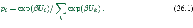
working opportunities at workplace ![]() . Then, an employee in household
. Then, an employee in household
![]() is assigned to a working opportunity at place
is assigned to a working opportunity at place ![]() with probability
with probability
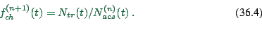
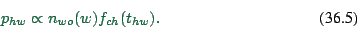
The complete approach works as follows:
(1) Synthetic population generation: First a synthetic population was generated based on demographic data (Beckman et al, 1996). The population data comprises microscopic information on each individual in the study area like home location, age, income, and family status.
(2) Compute the acceptance function ![]() . This is done
as follows:
. This is done
as follows:
(2.1) For each worker ![]() , compute the fastest path tree from
his/her home location. Compute the resulting workplace
distribution
, compute the fastest path tree from
his/her home location. Compute the resulting workplace
distribution ![]() as a function of trip time
as a function of trip time
![]() .36.2
.36.2
(2.2) Average over all these workplace distributions, i.e.
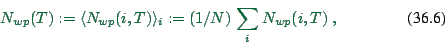 |
(36.6) |
(2.3) Compute the resulting average choice function via
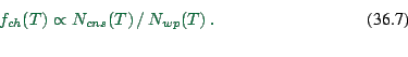 |
(36.7) |
 |
(36.8) |
(3) Assign workplaces. For each worker ![]() do:
do:
(3.1) Compute the congestion-dependent fastest path tree for the worker's home location.
(3.2) As a result, one has for each workplace the expected trip time
![]() . Counting all workplaces at trip time
. Counting all workplaces at trip time ![]() results in the
individual accessibility distribution
results in the
individual accessibility distribution ![]() .
.
(3.3) Randomly draw a desired trip time ![]() from the distribution
from the distribution
![]() .
.
(3.4) Randomly select one of the workplaces which corresponds to
![]() . (There has to be at least one because of (3.1).)
. (There has to be at least one because of (3.1).)
(4) Route assignment: Once people are assigned to workplaces, the simulation is run several times (5 times for the simulation runs presented in the paper) while people are allowed to change their routes (fastest routes under the traffic conditions from the last iteration) as their workplaces remain unchanged.
(5) Then, people are reassigned to workplaces, based on the traffic conditions from the last route iteration. That is, go back to (2).
This sequence, workplace reassignment followed by several re-routing runs, is repeated until the macroscopic traffic patterns remain constant (within random fluctuations) in consecutive simulation runs. For this, one looks at the sum of all people's trip times in the simulation. The simulation is considered relaxed when this overall trip time has leveled out.
Running this on a 250 MHz SUN UltraSparc architecture takes less than one hour computational time for one iteration including activity generation, route planning, and running the traffic simulator. The 70 iterations necessary for each series thus take about 4 days of continuous computing time on a single CPU.
![\includegraphics[width=0.8\hsize]{iteration5-fig.eps}](img894.png)
|
 \, f_{ch}(t).
\end{displaymath}](img870.png)