It was already pointed out in Sec. 17.3 that
important real world quantities for traffic are flow and density. A
third quantity is speed. In fact, there are two different ways to
measure traffic: space-averaged measurements, and point (![]() spot)
measurements. The space-averaged measurements are done at specific
points in time, and they correspond to what one is used to from, say,
fluid-dynamics. The point measurements are closer to what is measured
in reality: A sensor, e.g. an induction loop, usually covers only a
small amount of space. It is common use to average point measurements
over sometime
spot)
measurements. The space-averaged measurements are done at specific
points in time, and they correspond to what one is used to from, say,
fluid-dynamics. The point measurements are closer to what is measured
in reality: A sensor, e.g. an induction loop, usually covers only a
small amount of space. It is common use to average point measurements
over sometime ![]() , for example
, for example ![]() or
or ![]() .27.1 These differences are not particularly intereresting, but they are
necessary to avoid some caveats.
.27.1 These differences are not particularly intereresting, but they are
necessary to avoid some caveats.
The two measurements are:
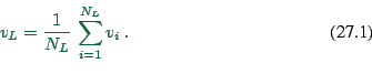 |
(27.1) |
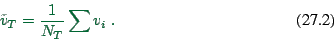 |
(27.2) |
Travel velocity ![]() is the more relevant quantity since
is the more relevant quantity since ![]() is the
time an average traveller needs for a distance
is the
time an average traveller needs for a distance ![]() . It is also the
quantity which is relevant for fluid-dynamical relations, for example
. It is also the
quantity which is relevant for fluid-dynamical relations, for example
![]() .
.
(also throughput). This is traditionally the most important
quantity, since it is easy to measure (one just has to count the
number of passing vehicles at a fixed location), and it is important
for the performance of the transportation system as a whole. In order
to allow comparison, it is often useful to divide flow by the number
of lanes. Say that during time ![]() we have measured
we have measured ![]() vehicles.
Flow then is
vehicles.
Flow then is
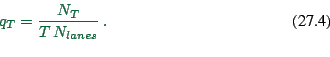 |
(27.4) |
Transportation science also uses the term volume. According to Gerlough and Huber (48), this should be reserved to hourly flows (i.e. measured over one hour and expressed in ``vehicles per hour''). Maximum flow is also called capacity.
There is no direct way to measure space-mean flow. However, sometimes
it is useful to use the relation ![]() . We then have
. We then have
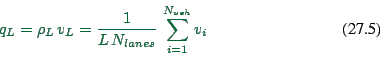 |
(27.5) |
Space-averaged density ![]() is the number of vehicles on a certain
stretch of road, divided by the length
is the number of vehicles on a certain
stretch of road, divided by the length ![]() of that stretch. In order
to allow comparison, it is useful to also divide by the number of
lanes:
of that stretch. In order
to allow comparison, it is useful to also divide by the number of
lanes:
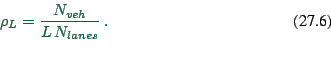 |
(27.6) |
Point density has no natural measurement. One can use
![]() .
.
An alternative method for point density is the ``fraction of time that
a sensor is covered by a vehicle'', also called occupancy.
Unfortunately, this quantity is difficult to obtain from a
time-discrete simulation. Since the duration a sensor is covered by a
vehicle is ![]() , the correct measurement in a simulation would
be [[check]]
, the correct measurement in a simulation would
be [[check]]
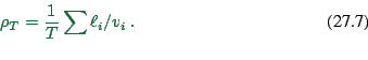 |
(27.7) |
![\includegraphics[width=0.8\hsize]{gz/synchronized_time.eps.gz}](img349.png)