Rules of the model

Single lane uni-directional traffic

Our traffic simulation is based on a cellular automata technique, i.e., a road is composed of cells, and each cell can either be empty, or occupied by exactly one vehicle (77,87), see Fig. 32.1 (a). Since movement has to be from one cell to another cell, velocities have to be integer numbers between 0 and $v_{max}$, where the unit of velocity is [cells per time-step]. It turns out that reasonable values are (87,9):

• length of a box $= 1 / \rho_{jam} =$ 7.5 m ($\rho_{jam} =$ density of vehicles in a jam).

• time step $=$ 1 sec

• maximum velocity $=$ 5 boxes per time step $= 5 \cdot 7.5~\hbox{m} / \hbox{sec} = 135 \hbox{km/h} \approx 85 \hbox{mph}$

For other conditions, such as higher or lower speed limits, this can be adapted.

Note that this approach implies a coarse graining of the spatial and temporal resolution and therefore of the velocities. A vehicle which has a speed of, say, 4 in this model stands for a vehicle which has a speed anywhere between $3.5 \cdot 7.5$ meters/sec $\approx$ 95 km/h (59 mph) and $4.49999 \cdot 7.5$ meters/sec $\approx$ 121 km/h (75 mph).

Vehicles move only in one direction. For an arbitrary configuration (velocity and position), one update of the traffic system consists of two steps: a velocity update step consisting of three consecutive rules, and a movement step according to the result of the velocity update. The whole update is performed simultaneously for all vehicles. The complete configuration at time step $t$ is stored and the configuration at time step $t+1$ is computed from that ``old'' information. Computationally we calculate in time step $t$ (with the three rules) the new velocity of each car and write this newly calculated velocity in the same site without moving the car (velocity update). After that we move all cars according to their newly calculated velocity (movement update).

1. (velocity update)

   For all particles $i$ simultaneously, do the following:

   IF ( $v_i \ge gap_i$ )

            $$v_i := \cases{ gap_i-1 & with probability $p_{noise}$\ if possible\footnotemark \cr gap_i & else \cr }$$ (close following/braking)

   ELSE IF ( $v_i < v_{max}$ )

            $$v_i := \cases{ v_i & with probability $p_{noise}$\ \cr v_i + 1 & else \cr }$$ (acceleration)

   ELSE (i.e. ( $v_i = v_{max}$ AND $v_i < gap_i$ )

            $$v_i := \cases{ v_{max}-1 & with probability $p_{noise}$\ \cr v_{max} & else \cr }$$ (free driving)

   ENDIF

2. (movement update)

   Move all particles $i$ to $x_i(t+1) = x_i(t) + v_i$.

The index i denotes the position (an integer number) of a vehicle, v(i) its current velocity, v$_{\it max\/}$ its maximum speed, gap(i) the number of empty cells ahead, and $p_{noise}$ is a randomization parameter.

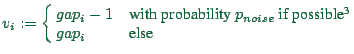
The first velocity rule represents noisy car following or braking. If the vehicle ahead is too close, the vehicle itself attempts to adjusts its velocity such that it would, in the next time-step, reach a position just behind where the vehicle ahead is at the moment. Yet, with probability $p_{noise}$, the vehicle is a bit slower than this.

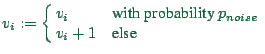
The second velocity rule represents noisy acceleration. Essentially, the acceleration is linear (i.e. independent from current speed), but with probability $p_{noise}$, no acceleration happens in the current time step (maybe as a result of switching gears etc.). Instead of an acceleration sequence of $0\to1\to2\to3\to\ldots$, a possible acceleration sequence can now be $0 \to 0 \to 1 \to 2 \to 2 \to 2 \to 3 \to \ldots$.

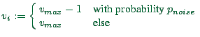
The last velocity rule represents free driving. Instead of remaining always at the same speed, such vehicles fluctuate between $v_{max}$ (with probability $1-p_{noise}$) and $v_{max} -1$ (with probability $p_{noise}$). Note that a vehicle which is set to $v_{max} -1$ will go through the acceleration step next time, thus in the next time step either staying at $v_{max} -1$ with probability $p_{noise}$ or getting back to $v_{max}$. Note that the resulting average speed of a freely driving vehicle is thus $v_{max} - p_{noise}$.

In terms of a microscopic foundation, the model is composed of the following elements:

• If a vehicle does not have enough space ahead, speed is proportional to space headway, which implies constant time headway (Pipes' theory, (73)).

• If there is enough space ahead for the given velocity, the vehicle accelerates linearly either to maximum speed or until the space headway becomes too small for further acceleration. A more realistic acceleration would probably be proportional to $1/v$, where $v$ is the speed. This would be computationally more burdensome; nevertheless, studies about the effect are under way. The effect on the principal traffic dynamics seem to be minimal (82).

• Deceleration is instantaneous within one time step. If one wants to constrain the model to realistic deceleration values, one needs to look at the velocity of the vehicle ahead. This is again computationally more burdensome, and the precise difference when changing this element alone with respect to the traffic dynamics is unclear (68) although it is clear that throughput will go up (11).

• On top of these rules, we add a fairly large amount of random noise in the velocity decision.

Somewhat shorter, the model enforces constant time headway for close following and for braking, but acceleration is ``delayed''. This puts the model into a large class of dynamically similar models which use ``time delayed'' constant time headway, e.g. of the type $a(t) \propto V[\Delta x(t)] - v(t)$ or $v(t+\tau) \propto V[\Delta x(t)]$, where $a$ is the acceleration, $v$ is the vehicle's velocity, $\Delta x$ is the space headway, $V(\Delta x)$ is a desired speed function, and $\tau$ is a time delay. It is certainly arguable that this does not catch all aspects of traffic; yet, all of these models are remarkably robust with respect to their traffic dynamics behavior, both in microscopic (6,78,68) and in fluid-dynamical (62,69) implementations.

Lane changing for passing

For multi-lane traffic, the model consists of parallel single lane models with additional rules for lane changing. Here we describe the two lane model which can be modified to any kind of multi lane model. Lane changing is modeled by an additional update step, which is added before the velocity update. The new sequence of steps is presented below. Steps two and three are the same in the single lane model and they are executed separately for each lane.

1. Lane changing decision
2. Velocity update
3. Vehicle movement

According to this lane changing rule set the vehicles are only moving sideways during the lane changing step; forwards movement is done in the vehicle movement step. One should, though, look at the combined effect of the lane changing and vehicle movement, and then vehicles will usually have moved sideways and forwards. The decision to change lane is implemented as strictly parallel update, i.e. each vehicle is making its decision based upon the configuration at the beginning of the update.

• Lane changing decision for passing
  • IF neighboring position $x_o(i)$ in other lane is vacant
    • THEN Calculate:
      • gap(i) Gap Forward in Current Lane,
      • ${\it gap_o\/}$(i) Gap Forward in Other Lane,
      • ${\it gap_b\/}$(i) Gap Backward in Other Lane,
      • IF (gap(i) $<$ v(i) AND ${\it gap_o\/}$(i) $> gap(i)$  )
        $\;\;\;\;\;-\;\;\;$THEN $weight1 = 1$
        $\;\;\;\;\;-\;\;\;$ELSE $weight1 = 0$
      • $weight2 = v(i) - gap_o(i)$
      • $weight3 = v_{max} - gap_b(i)$.
    • IF ( $weight1 > weight2$ ) AND ( $weight1 > weight3$ )^32.4
      • THEN mark vehicle for lane change^32.5

The rules are working in the following way (see Fig. 32.1 (b)): First we look at the neighboring position in the target lane. If this cell is vacant, we calculate the gap forward in the current lane ($gap$), the gap forward in the target lane ($gap_o$), and the gap backward in the target lane ($gap_b$). With these results we calculate the $weight1$ to $weight3$ described above. Finally if the weight comparisons render true the car will change to the new lane. After executing the lane changing decision we calculate the new velocity for all cars and move them according to this velocity.

This lane changing implementation follows a usual structure (110,50):

• Reason to change lanes? (Slow car ahead? Need to make turn later (see below)?)

• If yes: Target lane empty? (Definition of ``empty'' depends on ``urgency'')

• If yes: change lanes except for stochastic noise

Lane change implementations using this framework are remarkably robust in their dynamic behavior (102,110,90,50). This allows us, for example, not to look at other vehicle's velocities: The forward condition for the target lane, $gap_o \ge v$, is consistent with the condition $v \le gap$ for the car following; the backward condition for the target lane, $gap_b \ge v_{max}$ is simply a worst case scenario which nevertheless does not perform, in the analysis of the emergent properties, any worse than a condition which depends on the velocity of the other car (compare, e.g., (123) with (121)).

For three or more lanes, a simultaneous implementation of the lane changing decision can lead to collisions. For example, in a three-lane road two vehicles on the left and right lane could decide to go to the same spot in the middle lane. From an algorithmic point of view, this is possible because the lane changing decision is based on the configuration on time t; but it is also an entirely realistic situation.^32.6 To avoid collision we only allow lane changes in a certain direction in each time step:

• IF the time step is even

  THEN start procedure lane changing decision to the left for cars on the middle and then on the right lane

• IF the time step is odd

  THEN start procedure lane changing decision to the right side for cars on the middle and then on the left lane

Thus, left lane changes occur only on even time steps, right lane changes occur only on odd time steps. This behavior is collision free.

Lane changing for plan following

Vehicles in Transims follow route plans, i.e. they know ahead of time the sequence of links they intend to follow. This means that, when they approach an intersection, they need to get into the correct lanes in order to make the intended turn. For example, a vehicle which intends, according to its route plan, to make a left turn at the next intersection needs to get into one of the lanes which actually allow a left turn.

This is achieved in Transims by supplementing the basic lane changing rules with a bias towards the intended lanes. This bias increases with increasing urgency, i.e. with decreasing distance to the intersection. Technically, this is achieved by adding another weight to the acceptance conditions for lane changing:

• IF ( $weight1 + weight4 > weight2$) AND ( $weight1 + weight4 > weight3$)

  THEN change lane

$weight4$ is calculated according to

$$weight4 = \max\left[ { d^* - d \over v_{max} } , 0 \right]$$

for lane changes in the desired direction as long as the vehicle is not in one of the correct lanes, cf. Fig. 32.1 (c). $d$ is the remaining distance to the intersection, $d^*$ is a parameter; both are given in the unit of ``cells''. $d^*$ is currently set to 70 cells, i.e. approx. 500 m or 1/3 of a mile, throughout the simulation. In consequence, $weight4$ increases from zero to $d^*/v_{max}=14$ during the approach to the intersection. If $weight4 = 0$, then it does not influence lane changing decision. $weight4 = 1$ has the same effect as a slower vehicle ahead on the same lane. Further increases of $weight4$ more and more override the security criterions that the forward and the backward gap on the destination lane need to be large enough. $weight4 > v_{max}$ lets the vehicle make the lane change even if only the neighboring cell on the destination lane is free.

Once a vehicle is in one of the ``correct'' lanes within 70 cells (525 m) of the intersection, it is only allowed to change lanes if the target lane is also ``correct''. For movements that are allowed on multiple lanes through the intersection, this leads to equal usage of these lanes. This algorithm is not capable of leaving a single ``correct'' lane temporarily when encountering, say, a stopped bus on the same lane.

Unprotected turning movements

A necessary element of traffic simulations are unprotected turning movements. By this we mean that that for the movement the driver intends to make, some other lanes have priority. Examples are stop signs, yield signs, on-ramps, unprotected left turns.

The general modeling principle for this in Transims is based on a gap acceptance in the opposing (in Transims sometimes called ``interfering'') lanes, see Fig. 32.1 (d). Opposing lanes are the lanes which have priority; for example, for a stop-controlled left turn onto a major road this would be all lanes coming from the left plus the leftmost lane coming from the right. In order to accept the turn, there has to be a sufficient gap in each of these lanes.

Note that ``gap divided by the velocity of the oncoming vehicle'' is the oncoming vehicle's time headway, so the dynamics of this follows the Highway Capacity Manual (114). If one wants a time headway on an opposing lane of at least 3 seconds, then a vehicle with a velocity of 4 cells/second would have to be at least 12 cells away from the intersection.

The current Transims microsimulation uses a gap acceptance (gap between intersection and nearest car to the intersection which is approaching) of 3 times the oncoming vehicle's velocity, i.e. when the gap on each opposing lane is larger than or equal to the first vehicle on that lane, the move is accepted. For example, if the oncoming vehicle has a speed of 3, at least 9 empty cells have to be between the oncoming vehicle and the intersection. A special case is if the oncoming vehicle has the velocity zero, in which case no gap is necessary.

Signalized intersections

In Transims, we distinguish between signalized intersections and unsignalized intersections. In signalized intersections, the priorities are changing in time and regulated by signals. In unsignalized intersections, the priorities are fixed.

When a simulated vehicle approaches a signalized intersection, the algorithm first decides if, according to its current speed, it potentially wants to leave the link, i.e. its current speed (in cells per update) is larger than or equal to the remaining number of cells on the link.^32.7 If a vehicle wants to leave the link, the algorithm checks the ``traffic control'', which determines if the vehicle can leave the link. If it encounters a red light, it can not leave the link and no further action is taken. If it encounters a protected (green arrow) or caution (yellow) signal, the vehicle is allowed to enter the intersection. If it encounters a permitted signal (green, for example permitted left turn against oncoming traffic), the vehicle checks all opposing flows for a gap that is larger or equal to 3 times the oncoming vehicle's velocity (see Subsec. 32.4.4 above).

If the movement into the intersection is accepted, the vehicle is moved into an ``intersection queue''; there is one queue for each incoming lane. This queue models vehicle behavior inside an intersection. The vehicle gets a ``time stamp'', before which it is not allowed to leave the intersection; this time stamp is representative of the duration of the movement through the intersection. The intersection queues have finite capacity; once they are full, no more vehicles are accepted and the vehicles start to queue up on the link. This models the finite vehicle storing capacity of an intersection.

Once a vehicle is ready to leave the intersection, it moves to the first cell on the destination link if available. The speed of the vehicle is not changed when it is in the intersection queue so it exits on the destination link in the first cell with the same velocity that it had when it entered the queue.

Note that vehicles turning against opposing traffic make their decision to accept the turn when they enter the intersection queue, not when they leave it. This can have the effect that a vehicle enters the intersection queue when there is no oncoming traffic, but, because of other vehicles ahead of it in the same queue, cannot make its turn immediately. Yet, since the turn was already accepted, it will be executed as soon as all vehicles ahead in the same queue have cleared the queue and a cell on the destination link is available. The turn can occur during oncoming traffic. So in some sense vehicles will go ``through'' each other. Yet, note that on average the result is still correct. The approach described above will not let more vehicles through the intersection than a gap acceptance calculated when leaving the intersection queue. The above logic was chosen for simplification purposes since unsignalized intersections (see below) do not have queues and thus need to make their acceptance decisions when entering the intersection.

Unsignalized intersections

Unsignalized intersections in Transims have no internal queues, i.e. vehicles go right through them.^32.8 Also, vehicles leaving an unsignalized intersection go down the destination link as far as prescribed by their velocity, not just into the first cell as in the signalized intersections. Apart from these two differences, unsignalized intersections are similar to signalized ones.

When a simulated vehicle approaches an unsignalized intersection, the algorithm first decides if, according to its current speed, it potentially wants to leave the link, i.e. its current speed (in cells per update) is larger than or equal to the remaining number of sites on the link. If a vehicle wants to leave the link, the algorithm checks the ``traffic control'', which determines if the vehicle can leave the link. Currently occuring traffic controls are: no control, yield, and stop.

If a ``no control'' is encountered, the vehicle is moved to its destination cell without any further checks. For example, if a vehicle has a velocity of 5 cells per update and 2 more cells to go on its link, then it attempts to go 3 cells into the destination link. If that cell is already reserved (either by another ``reservation'' or by a real vehicle), then the next closer cell is attempted, etc., until the algorithm either finds an empty cell or returns that the destination lane is full. ``No control'' is usually used for the major directions, i.e. for the lanes which have priority.

If a yield sign is encountered, the vehicle checks the gap on all opposing lanes. According to the same rules as above, on all opposing lanes the gap needs to be larger or equal three times the first vehicle's speed on that lane. If the movement is accepted, the destination cell is selected according to the same rules as with the ``no control'' case.

If it encounters a stop sign, the vehicle is brought to a stop. Only when the vehicle has a velocity of zero for at least one time step on the last cell of the link is it allowed to continue. If the result of the regular velocity update indeed accelerates the vehicle,^32.9 then it attempts to go through the intersection. On all opposing lanes the gap, according to the same rules as above, needs to be larger or equal to three times the first vehicle's speed on that lane. If the movement is accepted, a vehicle coming from a stop sign will always go to the first cell on the destination link (if empty) and will have a velocity of one.

Parking locations

In the current Transims microsimulation, vehicular trips start and end at parking locations. Each link in the microsimulation, except for freeway ramps, freeway links, and some ``virtual'' links such as centroid connectors, has at least one parking location. Parking locations thus represent the aggregated parking options on that link. Parking locations have rules about how vehicles enter and exit the simulation:

• Each vehicle in Transims has a complete route plan, together with a starting time. At the starting time, the vehicle is added to a queue of vehicles that want to leave the same parking location. When the vehicle is the first one in the queue, it attempts to enter the link. The acceptance logic is in spirit similar to the logic of the unsignalized intersections, i.e. vehicles check the available gap and make their decision based on that. Parking accessory logic is not the focus of the current paper, and since that logic may change in Transims in the near future and we also expect no influence on the results presented here, we omit further technical details.

• A vehicle that has reached its destination parking location according to its plan will leave the microsimulation.

Parallel logic

Transims is designed to run on parallel computers, such as coupled workstations, desktop multi-processors, or supercomputers. The parallelization approach used for the microsimulation is a geographical distribution, i.e. different geographical parts of the simulated area are computed on different CPUs.

The current Transims microsimulation has these boundaries always in the middle of links. This is done in order to keep the complexity of the parallel computing logic as far away as possible from the complexity of the intersection logic.

Information needs to be exchanged at the boundaries several times per update in order to keep the dynamics consistent. For example, if a vehicle changes lanes and ends up close in front of another one, that other one is probably forced to brake. Now, if the lane changing vehicle is on one CPU and the following one on another, one needs to communicate the lane change. This will be called ``Update boundaries'' in the following section.

Complete scheduling

For a complete transportation microsimulation, we need to specify when movements are accepted, and also how conflicts are resolved. For example, vehicles simultaneously attempting to change lanes into the middle lane represent such a conflict. Another conflict is two vehicles from two different links competing for the same site on the destination link.

The complete update of the current Transims microsimulation is as follows. Assume that the state at time $t$ is the result of the last update. Let $t1$, $t2$, etc. be intermediate partial time steps.

1. Vehicles which are ready to leave intersection queues from signalized intersections reserve cells on outgoing lanes. They only attempt to reserve the first cell on the link; their velocity is the same as it was when they entered the intersection. When the cell is occupied (either by another ``reservation'' or by a vehicle), then the vehicle cannot leave the intersection. Note that there can be a conflict between different queues for the same destination cell. The current solution in Transims is that queues are served on a first come first served basis in some arbitrarily defined way, i.e. a queue which happens to be treated earlier in the microsimulation has a slightly higher chance of unloading its vehicles. -- Result: $t_1$ information.

2. Vehicles change Lanes. Use information from time $t_1$ to calculate situation at time $t_2$.

3. Exit from Parking. Results in $t_3$ information.

4. Exchange boundary information for parallel computing.

5. Non-signalized intersections reserve sites on target lanes. Note that there can be a conflict of two incoming links competing for the same destination cell. The current solution in Transims is that links are served on a first come first served basis, i.e. a link which happens to be treated earlier in the microsimulation has a slightly higher chance of unloading its vehicles. Note that this conflict only happens between minor links. Major links never compete for the same outgoing link except when there is a network coding error; and for the competition between major and minor links, the major link always wins because of the opposing lanes conditions.^32.10 Result: $t_4$ information.

6. Calculate speeds and do movements. If a vehicle scheduled for an intersection does not go through the intersection as a result of the velocity update, the reservation is cancelled. Vehicles which go through unsignalized intersections have $p$ set to zero, i.e. if it turns out that the result of the velocity update indeed brings them into the intersection, they need to go to the site on the destination lane which was reserved earlier. Result: $t_5 = t+1$ information.

7. Exchange boundary information and migrate vehicles for parallel computing.