Situation:
Have survey of ![]() persons, and options
persons, and options ![]() ,
, ![]() .
.
Also have attributes ![]() ,
, ![]() , ...
, ...
![]() as
well as
as
well as ![]() ,
, ![]() , ...
, ...
![]() .
.
[This means for example that we know the ``time by bus'' even if the person never tried that option.]
Note that we now have a person index ![]() everywhere.
everywhere.
Also have model specification
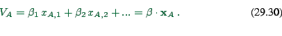 |
(29.28) |
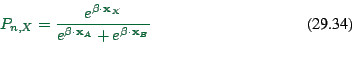
How to find
![]() ?
?
Assume set of persons ![]() that were asked.
that were asked.
![]() means person
means person ![]() chose option
chose option ![]() . (Implies
that
. (Implies
that ![]() .)
.)
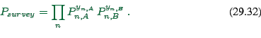
Assuming that we have our model, what is the proba that persons
![]() make choices
make choices ![]() ? It is (as usual,
assuming that the choices are indep)
? It is (as usual,
assuming that the choices are indep)
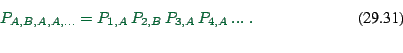 |
(29.29) |
Using the ![]() :
:
We want, via varying the
![]() , to maximize this
function.
, to maximize this
function.
In words, again: Want high probability that survey answers would come out of our model.
Maximizing in 1d means: Set first derivative to zero, and check that second derivative negative.
Maximizing in multi-d means: Set all first partial derivaties to zero; check that matrix of mixed second derivaties is negative semi-definite.
Instead of maximizing the above function, we can maximize its log
(monotonous transformation). Usual trick with probas since it
converts products to sums.
So far this is general; next it will be applied to Logit.
(Remember: ``Logit'' means ``Gumbel distributed randomness''.)
Strategy: Replace ![]() in Eq. (29.39) or in
Eq. (29.40) by specific from of logit model, i.e.
in Eq. (29.39) or in
Eq. (29.40) by specific from of logit model, i.e.
Computer science solution
From a computer science perspective, the maybe easiest way to
understand this is to just define a multidimensional function in the
variables
![]() and then to use a search algorithm
to optimize it.
and then to use a search algorithm
to optimize it.
This function would essentially look like
{}
double psurvey ( Array beta ) {
    double prod = 1. ;
    for ( all surveyed persons n ) {

        // calculate utl of option A:
        double utlA = 0. ;
        for ( all betas i ) {
            // utl contrib of attribute i:
            utlA += beta[i] * xA[n,i] ;
        }
        double expUtlA = exp( utlA ) ;

        // calculate utl of option B:
        double utlB = 0. ;
        for ( all betas i ) {
            // utl contrib of attribute i:
            utlB += beta[i] * xB[n,i] ;
        }
        double expUtlB = exp( utlB ) ;

        // contribution to prod:
        if ( person n had selected A ) {
            prod *= expUtlA/(expUtlA+expUtlB) ;
        } else {
            prod *= expUtlB/(expUtlA+expUtlB) ;
        }

    }
    return prod ;
}
Search algorithms could for example come from evolutionary computing.
The ``computer science'' way is almost certainly more computer intensive and less robust than the conventional strategy, lined out next. It does however have the advantage of being applicable also to cases where the conventional strategy fails.
Conventional strategy
The conventional strategy, mathematically more sound but also conceptually somewhat more difficult, is to first invest everything that one knows analytically and only then use computers.
The analytical knowledge mostly involves that one can search for maxima in high-dimensional differentiable functions by first taking the first derivative and then setting it to zero. This is lined out in the following.
Preparations
Define
![]() In consequence
In consequence
![]() and
and
![]() (Left version is sometimes useful.)
(Left version is sometimes useful.)
First derivative of ![]() :
:
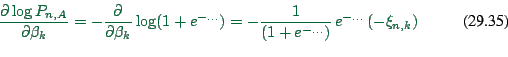 |
(29.33) |
We will also need
 |
(29.34) |
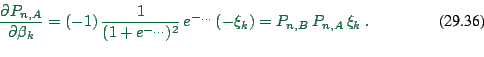
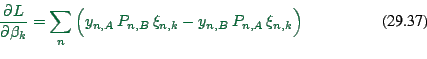
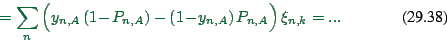
Core calculation
Now we can do
 |
(29.35) |
 |
(29.36) |
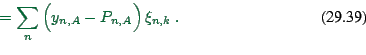 |
(29.37) |
(E.g. Newton in higher dimensions.)
Uniqueness (no contribution to understanding)
Need to check that this is a max (and not a min), and that it is the global max and not a local one.
Reminder: 1d function has max if 1st derivative is zero and 2nd deriv is negative. If 2nd deriv is globally negative, then this is the also the global max.
Translation to higher dimensions: Matrix of 2nd derivatives is globally negative semidefinite.
![]() negativ semidefinite:
negativ semidefinite: ![]() except for
except for ![]() .
.
Note: Assume ![]() . Then
. Then
![]() except for
except for ![]() as long as all entries of
as long as all entries of ![]() are real (i.e. not complex).
are real (i.e. not complex).
Now
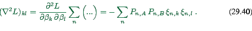 |
(29.38) |
Def
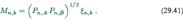 |
(29.39) |
Then
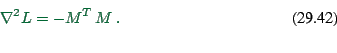 |
(29.40) |
Since all entries of ![]() are real,
are real, ![]() is positive definite,
and therefore
is positive definite,
and therefore ![]() negativ definite.
negativ definite.
![\begin{displaymath}
L = \log P_{survey}
= \sum_n [ y_{n,A} \, \log P_{n,A} + y_{n,B} \, \log P_{n,B} ] \ .
\end{displaymath}](img676.png)