Mobility Simulation

Selection of the pedestrian movement model

As mentioned above, the mobility simulation takes care of the physical aspects of the system, such as interaction of the agents with the environment or with each other. Typical simulation techniques for such problems are:

• In microscopic simulations, each particle is represented individually.

• In macroscopic or field-based simulations, particles are aggregated into fields. The corresponding mathematical models are partial differential equations, which need to be discretized for computer implementations.

• It is possible to combine microscopic and field-based methods, which is sometimes called smooth particle hydrodynamics (SPH; Gingold and Monaghan, 1977). In SPH, the individuality of each particle is maintained. During each time step, particles are aggregated to field quantities such as density, then velocities are computed from these densities, and then each individual particle is moved according to these macroscopic velocities.

• As a fourth method, somewhat on the side, exist the queuing simulations from operations research. Here, particles move in a networks of queues, where each queue has a service rate. Once a particle is served, it moves into the next queue.

For our simulations, we need to maintain individual particles, since they need to be able to make individual decisions, such as route choices, throughout the simulation. This immediately rules out field-based methods. We also need a realistic representation of inter-pedestrian interactions, which rules out both the queue models and the SPH models.

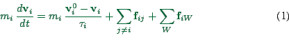
For microscopic simulations, there are essentially two techniques: methods based on coupled differential equations, and cellular automata (CA) models. In our situation, it is important that agents can move in arbitrary directions without artifacts caused by the modeling technique, which essentially rules out CA techniques. A generic coupled differential equation model for pedestrian movement is the social force model (Helbing et al., 2000)

$$%% nach Helbing 1:1, verwendet von LMauron und in pedsim m_i ... ... + \sum_{j\ne i}{\mathbf{f}_{ij}} + \sum_{W}{\mathbf{f}_{iW}}$$ (1)

where $m_i$ is the mass of the pedestrian and $\mathbf{v}_i$ its velocity. $\mathbf{v}_i^0$ is its desired velocity; in consequence, the first term on the RHS models exponential approach to that desired velocity, with a time constant $\tau_i$. The second term on the RHS models pedestrian interaction, and the third models interaction of the pedestrian with the environment.

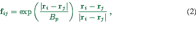
The specific mathematical form of the interaction term does not seem to be critical for our applications as long as it decays fast enough. Fast decay is important in order to cut off the interaction at relatively short distances. This is important for efficient computing, but it is also plausible with respect to the real world: Other pedestrians at, say, a distance of several hundred meters will not affect a pedestrian, even if those other pedestrians are at a very high density. We use an exponential force decay of

$$\mathbf{f}_{ij} = \exp\left(\frac{\vert\mathbf{r}_i - \math... ...}_i - \mathbf{r}_j}{\vert\mathbf{r}_i - \mathbf{r}_j\vert} ,$$ (2)

which seems to work well in practice. $\mathbf{f}_{ij}$ is the force contribution of agent $j$ to agent $i$; $\mathbf{r}_i$ is the position of agent $i$. Alternative more sophisticated formations are described by Helbing et al. (2000). For the environmental forces, $\mathbf{f}_{iW}$, the same mathematical form as for the pedestrian-pedestrian interaction is used.

Path following

The main problem with existing pedestrian models for our purposes is that they do not work when confronted with such large areas as are necessary to cover a complete hiking area: Covering an area of $(50 km)^2$ area (necessary to allow hikes of length $25 km$ in all directions from a central starting point) with cells of $(0.25 m)^2$ results in $10^{10}$ cells, which needs at least $40 GByte$ of memory. This makes the straightforward application of a technique based on cells impossible. Models based on continuous coordinates have the similar problem that all objects need to be represented, and again a straightforward implementation goes beyond available computer memory. All models have the problem that long-distance path following has never been looked at, at least not to our knowledge.

We introduced (Gloor and Nagel, 2002; Mauron, 2002) a model that uses only sparse information which fits into computer memory, runs efficiently on our scenarios, and has agents follow paths without major artifacts. This model will be described in the following.

For our simulation, we need to assume that the geometry is given by a graph (network) of hiking path plus some terrain features, and that the desired velocity of the hiker is consistent with this graph. The maybe first implementation that comes to mind is as follows:

• Make the desired velocity point directly to the next way-point: $\mathbf{v}_i^0 = v_i^0 (\mathbf{R} - \mathbf{r}_i)/{\vert\mathbf{R} - \mathbf{r}_i\vert} ,$ where $\mathbf{r}_i$ is the hiker's current position, $R$ is the position of the next way-point, and $v_i^0$ is the magnitude of the desired velocity. Once a way-point is reached, $\mathbf{R}$ is moved to the next way-point.

• Set the environmental force field to zero on the path, and such that it pushes the hiker back onto the path outside.

However, this approach has the disadvantage that, close to a way-point, agents are artificially pulled towards that way-point even if that does not make sense (see Fig.4). This could be avoided by switching to the next way-point before actually reaching this way-point, but then without special measures pedestrians may not be able to execute a switchback, because the next way-point may pull them back on the current segment. Also, the approach quite in general does not work once curved segments are allowed between way-points.

We developped a more specialized approach (Gloor and Nagel, 2002; Mauron, 2002), in which this artefacts do not exist. Our model uses a path-oriented coordinate system (see Fig. 5) for the computation of the desired velocity. It also uses a so-called path-force, which pulls the agents back on the path when he moves away from its center (e.g. due to interaction with other agents or obstacles). Fig. 6 demonstrates that the new approach keeps the pedestrians on their side of the path even in the vicinity of way-points.

Figure 4: Traces of hikers in the naive model, where they are all pulled towards the same way-point. Note how the trajectories focus near the way-point, and diverge before and after. The width of the path remains unchanged.

Figure 5: Path-oriented coordinate system for the computation of the desired velocity and the path forces. The light arrows show the desired velocity, which drives the agent forward along the path. The dark arrows show the path force, which pull the agent towards the middle of the path.

Figure 6: Traces of pedestrians walking in the same direction according to our model. Note that they stay on their side of the path, even at a bend.

Computational aspects

Figure 7: The hybrid simulation technique. The forces (arrows) are valid for the whole cell; a pedestrian's trajectory (dots) can follow arbitrary positions.

It was argued earlier that a cellular automata representation of space did not seem appropriate for our purposes, because of problems with off-axis movement. Instead, we use a continuous representation of space. However, some aspects of our simulation, like the calculation of forces that affect the agent, depend on the spatial location of the agent. These forces are relatively expensive to calculate, since one needs to enumerate through all possible objects that could influence a given location.

Yet, since those forces do not depend on time, they can be pre-computed before the simulation starts. In order for this to be successful, some coarse-graining of space is necessary. For this, we use cells of size $25cm \times 25cm$, and assume that all time-independent forces are constant inside a cell. The resulting force field (Fig. 7) becomes non-continuous in space, but this is not a problem in practice since this only influences the acceleration of pedestrians. That is, the acceleration contribution from the environmental forces can jump from one time step to the next, but since time is not continuous, this is not noticeable.

Precomputing the values for all cells in a hiking region of, say, $50km \times 50km$, does not fit into regular computer memory. To avoid this problem, we implemented two methods: lazy initialization, and disk caching. By lazy initialization, we mean that the values are computed only when an agent really needs them, also knows as Virtual Proxy Pattern (Gamma et al., 2001, pages 207-217). In practice, the simulation area is divided into blocks of size $200m \times 200m$. Every time an agent enters one of these blocks, the values for all cells inside that block are computed. Since hiking paths cross only a small fraction of those blocks, the cell values for many blocks in our hiking area will never be calculated.

In addition, the cell values, once computed, are stored on disk (disk caching). Every time when an agent encounters a block for which the cell values are not in memory, the simulation first checks if they are maybe on disk. Computation of the cell values is only started when those values are not found on disk. In consequence, a simulation started for the first time will run more slowly, because the disk cache is not yet filled.

If the simulation runs out of memory, then blocks which are no longer needed, i.e. which have not been crossed by an agent for a long time, are unloaded from memory. If they are needed again, they are just re-loaded from disk. This corresponds to the Least Recently Used (LRU) Page Replacement Algorithm described by Tanenbaum (2001, pages 218-222).

An additional advantage of the blocks, well known from molecular dynamics simulations, is that one can use them to cut off the short-range interaction between the pedestrians. Agents which are not in the same or one of the eight adjacent blocks are ignored. This implies that there needs to be some data structure where agents are registered to the block. Agents that move from one block to another need to unregister in the first block and register in the next one. In this way, an agent searching for its neighbors only needs to go through the registered agents in the relevant blocks. This brings the computation complexity from O($N^2$) down to O($N\!M$), where $N$ is the number of all agents in the simulation, and $M$ is the number of agents in a single block. $M$ is a reasonably small number when compared to the number $N$ of all agents in a real-world scenario.

For a testing scenario, of size $12 km \times 15 km$, we would need approx. $2.9 \times 10^9$ cells or $4500$ blocks, resulting in 9 GByte memory requirement. The result of the lazy initialization together with the caching mechanism is that 50 MByte are enough for the scenario shown in Fig. 11. The computational speed for that simulation, with 500 hikers, was about 100 times faster than real time.