QUEUE MODEL

Original Queue Model

Each link has, from the input files, the attributes free flow velocity $v_{0}$, length $L$, capacity $C$ and number of lanes $n_{lanes}$. Free flow travel time is calculated by . The storage constraint of a link is calculated as , where $\ell$ is the space a single vehicle in the average occupies in a jam, which is the inverse of the jam density. We use $\ell = 7.5~\hbox{m}$.

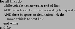
The intersection logic by Gawron (34) is that all links are processed in arbitrary but fixed sequence, and a vehicle is moved to the next link if (1) it has arrived at the end of the link, (2) it can be moved according to capacity, and (3) there is space on the destination link (Fig. 1(a)). The three conditions mean the following:

A vehicle that enters link $a$ at time $t_0$ cannot leave the link before time $t_0 + T_0$, where $T_0$ is the free speed link travel time as explained above.

The condition ``vehicle can be moved according to capacity'' is determined as

$$N < C ~~\hbox{or}~~\Big(N = C ~~\hbox{and}~~ rnd < f \Big)$$

where $C$ is the integer part of the capacity of the link (in vehicles per time step), $f$ is the fractional part of the capacity of the link, and $N$ is the number of the vehicles which already left the same link in the same time step. $rnd$ is a random number such that $0\leq rnd \leq 1$. According to this formula, vehicles can leave the link if the leaving capacity of the link has not yet been exhausted for this time step. If the capacity per time step is non-integer, then we move the last vehicle with a probability which is equal to the non-integer part of the capacity per time step.

``Space on destination link'': If the destination link is full, the vehicle will not move across the intersection.

Fair Intersections and Parallel Update

As discussed earlier, the problem with this algorithm is that links are always selected in the same sequence, thus giving some links a higher priority than others under congested conditions.

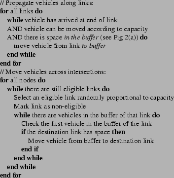
One can modify the algorithm so that links are prioritized randomly proportional to capacity. That is, links with high capacity are more often first than links with low capacity. In contrast to Ref. (4), we serve all vehicles of an incoming link once that link is selected.

To make this work, the algorithm was moved from link-oriented to intersection-oriented (that is, the loop now goes over all intersections, which then look at all incoming links), and we have separated the flow capacity constraint from the intersection logic. The latter was done by introducing a separate buffer (see Fig. 2(a)) at the end of the link, which is of size $\lceil C_{link} \rceil$, i.e.first integer number being larger or equal than the link capacity (in vehicles per time step). Vehicles are then moved from the link into the buffer according to the capacity constraint and only if there is space in the buffer; once in the buffer, vehicles can be moved across intersections without looking at the flow capacity constraints. This approach is borrowed from lattice gas automata, where particle movements are also separated into a ``propagate'' and a ``scatter'' step (35).

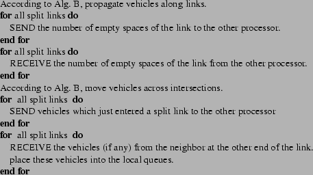
As a desired side effect, this makes the update in the algorithm completely parallel: If traffic is moved out of a full link, the new empty space will only open in the buffer and not on the link, and will thus not become available at the upstream intersection until the next time step - at which time it will be shared between the incoming links according to the method described above. This has the advantage that all information which is necessary for the computation of a time step is available locally at each intersection before a time step starts - and in consequence there is no information exchange between intersections during the computation of the time step. Further details are given in algorithmic form in Fig. 1(b).

In order to systematically test this intersection logic, an intersection test suite was implemented. This test suite goes through several different intersection layouts and tests them one by one to see if the dynamics behaves according to the specifications. The results typically look as shown in Fig. 2(b). In this particular example, one link with 500veh/sec and one link with 2000veh/sec merge into a link with a capacity of 500veh/sec. The curves are, for different algorithms, time-dependent accumulative vehicle numbers for the two incoming links. In this case, one sees that until approx time-step 3400, both links discharge at rates 400 and 100veh/sec, respectively. After that time, the first link is empty, and the second link now discharges at 500veh/sec. Not all algorithms are similarly faithful in generating the desired dynamics; the thick black lines denote results from the algorithm that got finally implemented. For further details, see (36).

Figure 1: (a) The original queue model. (b) Vehicle movement at the intersections. Note that the algorithm separates the flow capacity from intersection dynamics. (c) Parallel implementation of queue model.

[]

Algorithm A - Handling Constraints - Original algorithm

[]

Algorithm B - Links and Intersections separated:

[]

Algorithm C - Parallel computing implementation