Computational techniques

Introduction

As mentioned at the end of the last section, an agent-based approach to travel behavior simulations leads to a large number of heterogeneous modules that need to coexist in a joint simulation environment. This raises many questions about computational implementation, such as:

• Authoring: heterogenity of models implies that different people will need to cooperate on multi-agents simulations. What are the coding tools and policies needed?

• Data management: storing the initial conditions as well as the performance of the physical layer and the agent decisions needs to be coordinated. Are the existing systems appropriate for these outputs?

• Module coupling: heterogenous modules have to agree on some protocols and some data exchange. A lot of todays' computing research is concerned about this. Which techniques are available in our case?

• Performances: realistic systems have million of agents. Even simple computations at the agent level (e.g. 10 seconds) will produce simulations that are prohibitive in term of CPU usage. Can parallelization and distributed computing help to reduce the simulation time?

These questions are the topic of this section.

Coding

Computing in the area of transportation deals with entities which are plausibly encoded as objects. Examples are travelers, traffic lights, but also links ($=$ roads) and nodes ($=$ intersections). This suggests the use of object-oriented programming languages, such as C++ or Java.

Object-oriented languages and inheritance

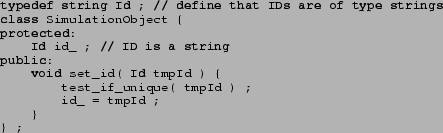
An important issue with the use of object-oriented programming languages is the use of inheritance. It is straightforward to start out by just having different computational classes for different classes of objects, for example for travelers, traffic lights, links, nodes, etc. However, eventually one will notice that those different classes share some similar properties. For example, they all have a unique identification tag ID, and it gets tiresome to reprogram the mechanics for this anew every time a new class is started. This implies that there should be a class SimulationObject that knows how to deal with ID tags. In C++, this could look as follows:¹

This could be used via

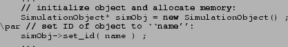
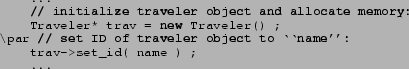
A traveler class could then inherit that functionality:

and without any further ado one could program

This becomes of particular importance if one needs different representations of the same entities for different purposes. For example, a link inside a simulation needs to be able to have a traffic dynamics executed on top of it, which implies that it needs some representation of road space. In contrast, a link inside a shortest-path computation will not need any of this, but it may need to be aware of time-dependent link travel times. The same is true if one wants to experiment with different models: Some behavioral model of a traveler may need the age of the traveler, while some other behavioral model may be interested in driver license ownership.

To a certain extent, it is possible to live with classes that are just supersets of all these properties. For example, if a traveler class already exists and contains an age variable, then driver_license_ownership could just be added. There are however cases where just adding variables causes too heavy burdens on computer memory consumption, such as when two researchers want to experiment with different mental memory models inside a traveler object. In such a case, both researchers can agree to use the same base class, which provides basic functionality including, for example, reading demographic properties from file, but then both researchers inherit from this base class to have their own extensions. C++ allows multiple inheritance so that class Traveler can be both a SimulationObject and a DatabaseObject for example. Java allows only single inheritance.

Container classes

Another useful property of modern programming languages is that increasingly advanced data structures are available. The arguably most important data structures for the purpose of travel behavior simulation are the container classes, which contain and maintain collections of objects. For example, all travelers can be stored in a single vector or list container. These container classes take care of memory allocation, that is, one does not have to know ahead of time how many elements the container will maximally contain. An important functionality of container classes are so-called iterators, which allow to go through all objects in a container in a systematic way without having to worry about array boundaries or memory faults.

In C++ , these classes are supplied by the so-called Standard Template Library (STL). They are now included by default in most modern C++ compilers and do not need any additional compiler switches any more. In Java, the container classes and related algorithms known as the Collections Framework have been around since the 1.2 release. The main difference between the C++ and the Java implementation of container classes is type safety: in C++ the compiler checks that objects from different types are not mixed up in a given container. In Java, object types are only checked during run time so that potential errors might still subsist in the code. The elaborated handling of exceptions in Java often allows the developer to track these errors in the early stage of development. Nevertheless, developers have since long recognized the advantage of generic programming offered by C++ templates. For this reason, a similar feature called Generics is going to be included in the next release (1.5) of Java (developer.java.sun.com/developer/technicalArticles/releases/generics/, accessed 2003).

Garbage collection

Some languages, notably Java, offer garbage collection, while some other languages, notably C++, do not offer it in their standard implementation. Garbage collection refers to a process that reclaims dynamically allocated but no longer needed memory during program execution. With multi-agent code, this could for example refer to an agent's plan which is no longer needed. A sophisticated implementation would explicitely put the previously needed memory into some pool of available free memory; but a less sophisticated or faulty implementation may forget this and for example just delete the pointer (i.e. the reference) to the memory location. Garbage collection in regular intervals goes through the memory and checks for areas to which no reference exists. Such memory areas are then moved into the pool of available free memory.

In multi-agent simulation code, in contrast to the typical numerical analysis application in FORTRAN for instance, objects are constantly created and destroyed because of the dynamic nature of the underlying model. Therefore, garbage collection and the absence of pointer arithmetics reduces by a large amount the debugging process since memory allocation bugs are the most frequent coding errors. However, garbage collection is usually slower, even though it can run in a parallel thread which helps on a multi-CPU machine.

Swarm/RePast

Some researchers in travel behavior research use the Swarm (www.swarm.org, accessed 2003) library. A similar but newer approach is RePast (repast.sourcefourge.net, accessed 2003). An advantage of RePast when compared to Swarm is that it is based on a wide-spread programming language (Java), in contrast to Swarm which is based on Objective C. Both approaches, and probably many others, provide library support to program systems which are composed of many agents or small software entities. The arguably most important element of support is the spatial substrate (e.g. cells, graphs, different types of boundary conditions). The provided functions include moving agents, checking for the presence of other agents, and, importantly, graphical output. In addition, the systems provides a mechanism to change parameters while the program is running (rather than having to edit some configuration file, or to re-compile the code). Support for data output and graphs is included.

Our own experience with these systems is that they are extremely useful in the prototyping of new models but potentially slow. This is certainly true when graphics is switched on, but it is probably still true when it is switched off. The reasons are that RePast uses a very nice object-oriented design that sometimes makes compromises with respect to computational performances and also that Java (the basis for RePast) is usually somewhat inferior to C++ in term of computational speed.

Readability and maintainability

An issue with object-oriented programming is code readability and maintainability. It is often claimed that object-oriented code is easier to maintain than other code. This is not consistent with our own experiences, and this statement is valid in spite of documentation support systems such as javadoc (java.sun.com/j2se/javadoc, accessed 2003) or doxygen (www.doxygen.org, accessed 2003). In particular, newcomers to an object-oriented code need to possess considerable language knowledge and experience in order to do meaningful changes. It is maybe more correct to say that object-oriented programming helps a programmer who is very fluent and experienced both in the concepts and in the technical details, and who works with a given code over a long period of time. It does however not necessarily help a project which is maintained by less experienced programmers, or when programmers change often, or when there is a big difference in object-oriented design preferences from one programmer to the next. It seems to us that only consistent teaching, which develops norms for ``building'' programs (in the same way as there are norms for planning and building bridges), will in the long run improve the situation.

Portability

Yet another issue contains portability. At this point, the only nearly completely portable language is Java, and it is portable even with graphics. One can only hope that Microsoft will continue to support a completely standard-conforming Java.

Regarding C++, as long as code is written without any graphical items such as user interfaces or graphical display of results, it is in principle possible to keep it portable between Unix, Windows, and Mac. (Since Mac OS-X is a Unix-based system, portability of Unix-based codes to and from Mac OS-X has become rather straightforward.) Nevertheless, our experience is that porting C++ code from Linux to Windows, even when it was written with portability in mind, takes several days, and the result is not entirely satisfying, since Unix uses Makefiles while Windows uses ``projects'' to organize large projects.

If one wants to deliver a Windows executable only, then the Cygwin (www.cygwin.com, accessed 2003) development environment may be a solution. The cygwin library comes as a Windows DLL (Dynamically Loaded Library) that wraps most of the standard Unix system calls and uses Windows system calls instead. The Cygwin development environment offers exactly the same tools as a Unix platform (bash, make, libc, gcc, g++, STL), but it does not provide an easy solution when someone wants to deliver a library or code that can be imported into a Windows IDE (Integrated Development Environment). Moreover, code that is sensible to the operating system layer will not be ported easily (e.g. socket I/O).

Computational performance

Common belief is that Java is considerably slower than C or C++. At least in the area of multi-agent traffic simulations, this is not consistent with our own observations. We have taught a class on multi-agent transportation simulations several times, which consisted of programming a simple traffic micro-simulation, a time-dependent fastest-path router, and a simple departure time choice model. With about half of the students programming in C++ and another half programming in Java, we rarely found important differences in terms of computational performance between the groups. The main differences that we have found are:

• Java often offers several methods to achieve similar things, for example different methods for I/O, e.g. reading and writing files. There is ample documentation in order to select which method solves which problem best, but we have found very little documentation with respect to the performance differences of those different methods. As understandable as this is from the perspective of robustness (``leave it to the compiler'' and ``technologies may change anyway''), this is not acceptable when file reading times can vary between several seconds and ten minutes, depending on the method that was selected.

• Message-passing libraries, such as MPI (see Sec. 3.6.3) are not well supported under Java: Despite some projects there is no standard, and support for special hardware such as Myrinet (see 3.6.1) is weak. This makes high performance parallel computing difficult with Java. On the other hand, there are emerging Java technologies such as Java Jini or Java RMI (Remote Method Invocation) that may be extremely appropriate for the immplementation of the strategy simulation layer since they allow, not only to move data accross computing nodes, but also code. However, the standard implementation of RMI suffers from large latencies (long start-up times before the first bit of a message is actually transmitted). Several projects have attempted to replace the communication layer with a high performance package to deploy RMI on clusters. See Secs. 3.6 and 3.7 for more information.

• In the past, high performance 3d graphics was not a strong point of Java. The Java3D package (java.sun.com/products/java media/3D, accessed 2003) is now more mature and it delegates most of the 3D intensive work to native libraries (such as Direct3D or OpenGL), that in turn delegate some of the workload to dedicated hardware. In practice, except for games and immersive simulations, Java can now be used to design medium-sized 3D applications such as used in CAD and scientific visualization.

Search methods

All the strategic parts of a travel behavior simulation are concerned with search: Finding links that combine to a good route; finding activity locations that suit individual preferences and constraints; finding good activity times; finding a residential location; etc. And many areas in computer science are indeed concerned with search. This reaches from purely engineering issues (``how to find a file on a hard disk'') via operations research (e.g. traveling salesman problem) to cognitive modeling and Artificial Intelligence.

For travel behavior research, it is important to know these methods, since many models in travel behavior research essentially lead to search problems that cannot be solved within reasonable time on existing or future computers. Take nested logit models, which can be visualized as a decision tree. For example, one can phrase activity-based demand generation as a nested problem, consisting of pattern choice, location choice, time choice, and mode choice (e.g. Bowman, 1998). An agent faced with the activity scheduling task first makes the pattern decision, then the location decision, etc. The decision at each level depends on the expected utility of each sub-tree. This means that, in order to compute the decision, one needs to start at the bottom leaves and iteratively propagate the utilities to the upper branches.

To understand this, let us index patterns with $p$, locations with $l$, times with $t$, and mode with $m$. The utility of a complete decision is denoted $U_{pltm}$. Now, for a given $plt$, the algorithm evaluates the different utilities for all $m$, and from that computes the expected utility for the choice $plt$. And here lies an important difference between different choice models: While in most computer science search algorithms, this would just be the maximum utility (i.e. $U_{plt} = \max_m U_{pltm}$), in random utility theory it is the expected maximum utility. For nested logit models, this is the famous logsum term $U_{plt} \propto \ln \sum_m e^{U_{pltm}}$.

The algorithm then computes utilities for all $t$ given $pl$, and from that computes the expected utility for the choice $pl$. This continues until the computation has reached the root of the decision tree. At this point, the algorithm turns around and goes down the decision tree, at each decision point making the best choice. Again, in computer science search, this choice would just be the best option, while in nested logit, an option is chosen with a probability proportional to $e^{\beta U_i}$.

This seemingly small difference between ``selecting the max at each decision point'' and ``selecting according to $e^{\beta U_i}$ at each decision point'' has very important consequences in terms of the search complexity: While the choice of the maximum allows to cut off branches of the search tree that offer no chance of success, in probabilistic choice all branches of the search tree need to be evaluated. This means that many efficient computer science methods cannot be used for random utility theory. More distinctly, evaluating a model using random utility theory is much more costly than evaluating a model using plain maximization. Now since many of the behavioral search problems cannot even be solved optimally using ``max'' evaluation, there is little hope that we will be able to directly solve the same problems using the even more costly random utility framework.

In consequence, at this point it makes sense to look at alternatives, such as the following:

• Sometimes, it is possible to use max-based search algorithms to compute not just the best option, but also second-best, third-best, etc. This is for example well known for shortest path computations (e.g. Perko, 1986). That is, one could limit the choice set to some $k$-best options.² In many cases, however, computing a second-best option is much more expensive than computing the best option.

• Random utility is in effect a noise parametrization: Agents do not compute the utilities that the scientists compute, but modify them by some random disturbances. However, stochastic simulations change from one iteration to the next anyway; that is, computing the fastest path based on each of the iterations of a Dynamic Traffic Assignment will generate a choice set, with different frequencies for each option. It would be interesting if this feature could be exploited, rather than trying to fight it as what is currently done by first averaging over many iterations to obtain a deterministic result and then use random utility modeling to re-introduce the noise.

• Computer science knows many search heuristics. These heuristics come up with useful solutions within limited resources; sometimes, they come together with some quality guarantee (such as ``not more than 10% worse than the optimal solution, even if we cannot compute the optimal solution''). Now, from a behavioral point of view, it seems that when a computer cannot reliably find an optimal solution, it is improbable that humans can do so. In consequence, it would make sense to look at computer science heuristics, and to compare them to heuristics based on human psychology.

  In this context, note that route choice is maybe not a good field to explore this since route choice is one of the few fields where the optimal solution, albeit maybe not behaviorally realistic, is extremely cheap to compute, much cheaper than most heuristic solutions.

A relatively new set of heuristic search algorithms are ``evolutionary algorithms''. This is a field that looks at biology and evolution for inspiration for search and optimization algorithms. Examples are Genetic Algorithms (Goldberg, 1989), Neural Nets, Simulated Annealing, or Ant Colony Optimization (Dorigo et al., 1999). These algorithms compete with methods from Numerical Analysis (such as Conjugate Gradient) and from Combinatorial Optimization (such as Branch-and-Bound). In our experience, the outcome in these competitions is consistently that, if a problem is well enough understood that methods from Numerical Analysis or from Combinatorial Optimization can be used, then those methods are orders of magnitude better. For example: There is a library of test instances of the traveling salesman problem (www.iwr.uni heidelberg.de/groups/comopt/software/TSPLIB95/, accessed 2003), and there is a collection of the computational performances of many different algorithms when applied to those instances (www.research.att.com/ $\!$dsj/chtsp/, accessed 2003). The largest instances of the traveling salesman problem that a typical evolutionary algorithm solves, using several hours of computing time, are often so small that a Combinatorial Optimization algorithm solves the problem in so short a time that is is not measurable.

In contrast, evolutionary algorithms are always useful when the problem is not well understood, or when one expects the problem specification to change a lot. For example, an evolutionary algorithms will not complain if one introduces shop closing times into an activity scheduling algorithm, or replaces a quadratic by a piecewise linear utility function. Faced with such problems, the evolutionary algorithms usually deliver ``good'' solutions within acceptable computing times and with relatively little coding effort.

This characterization makes, in our view, evolutionary algorithms very interesting for travel behavior research, since both according to random utility theory and according to our own intuition, this is exactly what humans do: find good solutions for problems within reasonable amount of time, and consistently find such good solutions even when circumstances change.

An interesting research issue would be to explore the distribution of solutions in the solution space. Maybe there are evolutionary algorithms that generate solutions of quality $U_i$ with probability $e^{U_i}$, but in much less time than the full search algorithm.

Databases for initial/boundary conditions

The necessity of initial and boundary conditions was described in Sec. 2.1. There is probably very little debate that databases are extremely useful to maintain information such as road network information or census data. There are now many commercial or public domain products which support these kinds of applications. Standard databases are always easy to use when the data consist of a large number of items that all have the same attributes. For example, a road link can have a from-node, a to-node, a length, a speed limit, etc.

The two most common situations are that of a GIS database and that of a database management system (DBMS) using an SQL relational database. Note that most GIS vendors provide gateways to link their software to SQL DBMS. Besides data management issues, the main advantages of using SQL DMBS is their flexibility. Data can exported and imported between simulation modules that are totally independent and useful statistics can be extracted very easily. URBANSIM (Waddell et al., 2003) and METROPOLIS (de Palma and Marchal, 2002) use that approach to store input and output data. The performance bottleneck of SQL DBMS is often the sorting of records and the insertion of new records. When these individual operations are performed at a very high rate, such as inside a simulation loop, the usage of a SQL DBMS severly deteriorates the overall performance. But when these operations are performed in bulk, these systems can be very efficient. For instance, at the end of a METROPOLIS simulation, the insertion of 1 million agents with 15 characteristics each in the underlying MySQL database takes only 2 sec. on a Pentium 4. MySQL (www.mysql.com, accessed 2003) is fast becoming a de facto standard because it is open-source, easy to manage, performant and it already integrates some geographic features of the OpenGIS specification (www.opengis.org, accessed 2003).

However, even the data for initial and boundary conditions is not entirely static. Changes can happen for the following reasons:

• Keeping it current: As time moves on, new streets are built and older ones are changed to pedestrian zones. The database needs to keep track of these changes.

• Errors: Any data contains errors, and all data including the historical data should be continuously improved over time.

• Higher detail: Data can be enhanced or replaced by data of higher detail. This could for example mean the inclusion of low capacity roads, the addition of public transit, higher resolution for the census data, or any other information.

• Scenarios: Most simulation applications in traffic refer to case studies, where some elements of the scenario are changed while all others are kept fixed. For example, a street could be added to or removed from the road network data, while all other data remain fixed.

Differences to ``standard'' database applications

The arguably main commercial application of standard databases are financial transactions. The task of such a system is to maintain a consistent view of the whole system at each point in time, to do this in a very robust way that survives failures, and to maintain a record of those states and the transactions connecting them.

Database applications for initial and boundary conditions are, in contrast, rather different. Our data is not defined by the transactions; rather, transactions are used to define the data. That is, a standard database will solve the problem of keeping the data current, but it will not solve the problem of retro-active changes, which are imposed by error corrections, higher detail imports, or scenarios. There seems to be very little database support for such operations. Some examples:

• Just replacing supposedly erronous data entries by supposedly more correct ones is not a viable option since in the long run nobody will know any more to what status the data corresponds. Any change in an existing data set needs to be documented; as a minimum requirement, there should be a complete trail of all changes together with the data of change and the name of the person doing the change.

• Changing data entries during the course of a case study is not possible, because simulation runs would no longer be comparable. This refers even to the correction of (supposedly) erronous data items: If a study was started with certain errors in a data set, it will have to be finished with those same errors.

  This makes it impossible to keep a database up to date while some other team is using it to run a study. The record and production of snapshots of the database is thus a crucial feature.

Diligence and discipline by the operators can overcome some of these issues. Records can contain fields which denote their temporal range of validity. For example, if a road link gets converted into a pedestrian link at the end of the year 2000, the whole link record in the database could be copied, the copy could be modified to reflect the new status, and then the first record could be marked as being valid until the year 2000, while the second record could be marked as being valid starting in 2001. Scenarios could be treated in a similar way, that is, the database contains a superset of all information ever used in the whole study, and flags denote which information is switched on or not for each specific case. The German company PTV has used a similar technique for the computation of all scenarios for the so-called Bundesverkehrswegeplan (Vortisch, personal communication).

When thinking about this, one recognizes that a similar mechanism needs to be employed for error correction. Essentially, it is necessary that data entries are never deleted. If one wants to correct supposedly erronous data entries, then the whole record needs to be copied, in the copy the erronous is corrected, and flags are adjusted so that the situation is clear. In that way, a study relying on the faulty record can still use that faulty record until the whole study is finished.

Version control systems

Now while it is clear that the above is feasible, it is also clear that it will be prone to errors. In particular, there is the all-too-human tendency to correct errors without telling anybody. In consequence, some software support for these operations would be useful. With current databases, it is possible to maintain a log of all operations, and so it is in principle possible to go back and find out who changed which entry when. This is however not sufficient: What is needed is a system that allows us to retrieve some data in the status it was at a certain point in time, no matter what the later changes are. And in fact, there are systems which do exactly what we want, but unfortunately only for text files and not for databases. These systems are called version control systems, and they are for example used for software development. The ``change log'' system of some text processors such as MS-Word and Openoffice is a related, albeit simpler system. An example of a version control system is CVS (www.cvshome.org, accessed 2003); it has the advantage that it works across different operating systems and that it allows remote access. Nearly all public domain software these days uses CVS.

Version control systems provide the following functionality:

• There is a main trunk of development. All changes that anybody ever does to the main trunk are recorded, together with a date, user name, and an optional comment.

• There is the option of branches. The typical use for branches are patches for stable software releases. Say that a software is released and used by others, while the main trunk goes into an experimental development phase. If at this point bugs are found in the released version, it will not be possible to fix those bugs in the experimental version and release that to users. Instead, one will make a branch which starts at the released version, and just do small patches to that version.

• Last, there is the option of merges. For example, in the above example it is possible to merge the patches into the experimental version.

• CVS also offers concurrent development, that is, more than one developer can work on the same files. For a variety of reasons, this is probably not relevant for the database issues discussed here.

The main point of shortly digressing into software version control systems is to show that systems which have the desired functionality are in existence and have been used for many years. This implies that it is a technology which is well understood and more than ready for release. The main reason why there seems no widespread use of version control technology in the database area is that the main customer of the database industry is the financial services industry - and that industry is mostly interested in a consistent view of the current situation, and not in the running of different scenarios. It is sincerely hoped that this situation will change in the future, and that some databases will be geared more towards scientific applications. Since other scientific areas, such as bio-informatics or high energy physics, are now moving into the wide-spread use of large scale databases, there is hope that this will happen soon. If it does not happen, then the transportation community should get together and design at least some minimal version, which would essentially be an ``add-only'' database, where entries, once entered, can never be removed. They could only be invalidated by a flag.

What to store/data aggregation

In our view, it makes sense that the primary data for initial and boundary conditions is as close to the physical reality as possible, since in our view that is the best way to obtain an unambiguous description. For example, it makes more sense to store ``number of lanes'', ``speed limit'', and ``signal phases'', rather than ``capacity'', since the latter can be derived from the former (at least in principle), but not the other way round. In part, this will be imposed to the community by the commercial vendors, which have an interest to sell data that is universally applicable, rather than geared to a specific community.

If the primary source of data is highly disaggregated, it is tempting to keep this high level of detail all through the forecast models, and projects such as TRANSIMS, METROPOLIS, and MATSIM develop large-scale simulation models that may, in the long run, be able to cope with highly disaggregated data for the physical layer and thus avoid any aggregation. However, this is not always feasible from the computational point of view, and therefore systems that run on more aggregated data will continue to exist. Unfortunately, the aggregation of much of traffic-related data is an unsolved problem - while it is straightforward to aggregate the number of items in cells in a GIS to larger cells, aggregating network capacity to a reduced graph is far from solved. There needs to be more research into multi-scale approaches to travel behavior simulations.

Even if these problems get eventually solved, we firmly believe that models should make the aggregation step transparent. That is, there should be universally available data, which, for the ambiguity reasons stated above, should be as disaggregated as possible, and then aggregation should appear as an explicit feature of the model rather than as a feature of the input data. Conversely, the results/forecasts should be, if possible, projected back to the original input data.

Data merging

Another issue with respect to databases that probably many of us have faced is the merging of data sets. Let us assume the typical case where we have some large scale traffic network data given, and some sensor locations registered for that network. Now we obtain a higher resolution description of a smaller geographical area. One would like to do the following:

• Overlay the second data set on the first one. Remove the items from the original data set that are superceeded by the higher resolution set and stitch the road networks together.

• Move the registration of the sensors, where applicable, to the new data set.

It would be possible to write heuristics which could solve most of the problem semi-automatically, i.e. in a way where uncritical cases are resolved automatically, and problematic situations are automatically presented to an analyst. This would be similar to the automatic proof checking technology applied in some software projects. However, to our knowledge, no such technology is available for transportation data.

The possible role of commercial data vendors

Some of the problems of data consistency will go away with the emergence of a few internationally operating data vendors. They will define the data items that are available (which may be different from the ones that we need), and they will make consistent data available at pre-defined levels. For example, it will be possible to obtain a data set which contains all European long-distance roads, and we would expect that it will be possible to obtain a consistent upgrade of the Switzerland area to a higher level of detail.

We are a bit more skeptic towards the commitment of such companies to historical data. With little cost, companies could make snapshots of the ``current view of the current system'', and one could thus obtain something like the ``year 2000 view of the year 2000 system''. There would, however, also be the ``current view of the year 2000 system'', or ``intermediate views of the year 2000 system''. The first would be useful to start a historical study; the second would be useful to add data consistently at some later point in time.

Finally, there will probably always be local error correction of the type ``company XY always gets A and B wrong and so we always correct it manually''. Obviously, such changes need to be well-documented and well-publicized.

Scenario maintenance

In our view, there is no system that manages the scenario data changes consistently as outlined above; in consequence, there is also no simulation system that manages consistently dependencies of simulation result on input data. A system should at least be able to remember what has happened to the data and what part of the forecast it affects. Some transportation planning software systems have made progress in that direction, e.g. EMME/2 and METROPOLIS.

EMME/2 (INRO Consultants Inc., 1998) comes with a binary-formatted, proprietay database (the so-called databank file). This file contains the description of the transportation network (links with lanes, length, capacities) and the travel demand in the form of OD matrices. EMME/2 proposes the definition of scenarios that consist in pairing networks and matrices and performing the assignment. EMME/2 designers recognized earlier the importance of tracing back all the modification done to the complex network layer: each change of a single attribute of the links is recorded and can be brought back. This feature is reminiscent of the roll-back feature of relational databases. However, once an assignment is performed, the output variables (here the traffic volumes) do not follow the same handling: these variables are erased after each assignment and have to be kept manually in user-defined vectors. The modifications of the initial data does not invalidate the results. However, EMME/2 provide the feature of multiple scenarios so that the end-user can modify the network of another scenario, run the assignment, and compare the scenarios. It is left ot the discipline of the user not to modify the initial data thereafter.

METROPOLIS use the same network description (not storage) as EMME/2. It uses also an OD matrix but with an extra layer of agent description called ``user types'' that define user constraints in term of schedule. METROPOLIS uses an open SQL relational database (MySQL) to store all the initial data it needs: networks, matrices, users, scenarios. The roll-back feature is delegated to the database. The idea is that, even if it useful to be able to roll-back, it is often unusable when the number of components that have changed is huge. For instance, if all the capacities of the network are multiplied by 1.1, it will not be possible to understand the modifications unless it is documented with a log. However, METROPOLIS maintains the consistency of data throughout the simulation process: no data can be modified that have been used in a completed simulation. METROPOLIS distinguishes different bulks of data sets: networks, matrices, user-types, function sets, demands, supplies and finally, simulations (Fig 4). Each of these major blocks encapsulates a whole set of disaggregated data (e.g. networks have thousands of links). This decomposition is arbitrary and only intented to ease the use of creating scenarios by mixing variants. Each of these data sets can be in one of the 3 different states: free, editable or locked. In the free state, the data block can be erased/modified without compromising results or other data sets. In the editable state, other data blocks depend on this one and so this one cannot be deleted without deletion of the dependent blocks; however no simulation has been performed using it and it can still modify its internal attributes. In the locked state, it means that some simulation has been or is using the data set and so the data set cannot be modified. By doing so, the METROPOLIS inner database ensures that whatever results is still in the database contains also the exact initial data set of the simulation. However, no log is kept of the modifications that might have been done to generate the initial set and it is left to the end-user to write something in the comment attribute of each data block. Each data block can be duplicated/deleted/documented to ease the replication of experiments and the comparisons between forecasts that share some data blocks.

Module coupling

Introduction

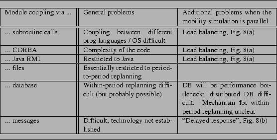
As pointed out earlier, multi-agent transportation simulation systems consist of many cooperating modules, such as the synthetic population generation module, the housing market module, the activity generation module, etc. An important issue for the future development of multi-agent transportation simulations is the coupling between those modules, i.e. how they cooperate to form a coupled simulation system.

Despite many efforts, the easiest solution in terms of the implementation of a simulation package is still to have a single person writing a complete system for a single CPU on a single operating system (OS). In addition, all tightly coupled modules should use the same programming language since that considerably simplifies the coding of module interaction.

With multi-person projects, the argument remains the same: The easiest approach is to program for a single-CPU system and have everybody use the same OS and the same programming language at least for tightly coupled modules. However, as models evolve, it is desireable to be able to plug-in new modules without compromising the whole architecture. This section will explore technologies for this purpose.

The coupling of the modules also depends on their synchronization. Obviously, the organization of how user decisions take place on the time scale affects considerably the way the modules will interact. When decisions are revised frequently in the simulation, it imposes to have a coupling implementation that is computationally efficient.

Subroutine calls

There are many ways to couple modules and all methods have their own advantages and disadvantages. The first one that comes to mind is to couple them via regular subroutine calls. For instance, the traffic ($=$ mobility) simulation can be suspended at regular intervals and each agent is asked if he/she wants to replan. If the answer is yes, the corresponding subroutine is called. Once all agents are treated, the system returns to the traffic simulation thread.

The advantages of this method are that it corresponds to long-established programming methods, and that its logical scheduling is easy, in the sense that while a traveler ``thinks'', the flow of the real world is suspended. This makes it rather easy to model all kind of thought models, including immediate or delayed response.

The disadvantages of this method are that the different methods need to be compatible on some level, which usually means that they are written in the same programming language on the same OS. In addition, the approach is not amenable to a parallel implementation, as will be discussed in Sec. 3.7.2. The more strategic modules one includes, the less time the CPU will have to advance the simulation of the physical system. Large scale scenarios are infeasible with this method.

Using files (including XML) to exchange information

Often, different strategy generation modules come from different model writers. Some group might provide a router, some other group an activity generation module, and the next group a housing choice module. All of these modules may be coded in different programming languages and on different OSs. For such modules, coupling via subroutine calls is no longer possible. In such a case, the maybe first thing that comes to mind is to couple them via files. This approach is in fact followed by many groups, including TRANSIMS and some of our own work.

A question here is which file format to use. TRANSIMS uses line-oriented text files. This works well as long as the data are column-oriented, such as files for links and nodes. It becomes considerably more awkward with respect to agent information, which is less well structured:

• Strategies of agents may contain variable-length pieces, such as a route. Also, there may be hierarchical information, such as demographic information (on the agent level), information about different alternatives, or information about every specific decision point.

• Not all agents may have the same information. This makes the column-oriented approach difficult, since for each additional information item a new column needs to be started, even if it remains unused by most agents.

A plausible way out of the dilemma is offered by the XML format (www.w3.org/XML, accessed 2003). Rather then dwelling on general descriptions, let us look at a possible example:

The example denotes a traveler agent with two plans, one with score ($\approx$ utility) of $561$ and one with score $463$. The first plan is given in more detail, it consists of an activity chain of ``home-work-home'', together with some location information whose exact type (e.g. street address, x/y coordinate, link ID) is not specified here. In addition, there is information on activity scheduling times, and on travel times.

The point here is not to debate the details of the data entries; the two important points are the following:

• Consolidated person information. All information about a person is at one place. In fact, in our own current work we just use one single file format to exchange agent information between all modules. Higher level modules, such as activity planning, may not need lower level information such as route information and thus they may ignore the corresponding fields or leave them empty. However, with this file format, all modules have always access to all information concerning an agent. For example, the routing module has access to the demographic data. This is in stark contrast to some earlier approaches, notably TRANSIMS, and it is in our view much more amenable to the agent-based view. It is also much more amenable to true behavior-based modeling.

• Extensibility. The ``X'' in XML stands for extensible. It is possible to add information into the above file without breaking existing parsers. This means that anybody can experiment with additional items to the format without having to adapt all other modules. It is correct that the same thing can be achieved, within limits, with a column-based format, but XML is certainly much more flexible and powerful in what it can do.

Somewhat contrary to expectations, file size with XML is not a major issue. Our own experience is that uncompressed XML files are larger than the corresponding column-oriented TRANSIMS files, but once compressed, the XML files are considerably smaller. We attribute this to the fact that repeated tags such as <person> are easy to compress, and to the fact that column-oriented files have the tendency to contain a lot of unnecessary ``zeroes'' since many of the columns may not be used by most of the agents.

The arguably easiest way to implement file-based module coupling is to do it together with period-to-period (e.g. day-to-day, year-to-year) replanning: The simulation of the physical system is run based on precomputed plans and the behavior of the simulation is recorded, some or all of the strategic modules are called, the simulation is run again, etc.

The file-based approach solves possible data exchange issues between different programming languages and different OS, but it does not solve the performance issue: The assumption is still that at any given point in time, only a single CPU is advancing the simulation. It is however possible to parallelize each individual module. This will be discussed in Sec. 3.6.

Remote procedure calls (e.g. CORBA, Java RMI)

An alternative to files is to use remote procedure calls (RPC). Such systems, of which CORBA (Common Object Request Broker Architecture; www.corba.org, accessed 2003) is an example, allow to call subroutines on a remote machine (called ``server'') in a similar way as if they were on the local machine (called ``client''). There are at least two different ways how this could be used for our purposes:

1. The file-based data exchange could be replaced by using remote procedure calls. Here, all the information would be stored in some large data structures, which would be passed as arguments in the call.

2. One could return to the ``subroutine'' approach discussed in Sec. 3.5.2, except that the strategic modules could now sit on remote machines, which means that they could be programmed in a different programming language under a different OS.

Another option is to use Java RMI (java.sun.com/products/jdk/rmi, accessed 2003) which allows Remote Method Invocation (i.e. RPC on java objects) in an extended way. Client and server can exchange not only data but also pieces of code. For instance, a computing node could be managing the agent database and request from a specific server the code of the module to compute the mode choice of its agents. It is easier with Java RMI than with CORBA to have all nodes acting as servers and clients and to reduce communication bottlenecks. However, the choice of the programming language is restricted to Java.

It is important to notice the difference between RPC and parallel computing, discussed in Sec. 3.6. RPCs are just a replacement for standard subroutine calls which are useful for the case that two programs that need to be coupled use different platforms and/or (in the case of CORBA) different programming languages. That is, the simulation would execute on different platforms, but it would not gain any computational speed by doing that since there would always be just one computer doing work. In contrast, parallel computing splits up a single module on many CPUs so that it runs faster. Finally, distributed computing (Sec. 3.7) attempts to combine the interoperatility aspects of remote procedure calls with the performance aspects of parallel computing.

The main advantage of using of CORBA and other object broker mechanisms is to glue heterogeneous components. Both DynaMIT and DYNASMART projects use CORBA to federate the different modules of their respective real-time traffic prediction system. The operational constraint is that the different modules are written in different languages on different platforms, sometimes from different projects. For instance, the graphical viewers are typically run on Windows PCs while the simulation modules and the database persistency are carried out by Unix boxes. Also, legacy software for the data collection and ITS devices need to be able to communicate with the real-time architecture of the system. Using CORBA provides a tighter coupling than the file-based approach and a cleaner solution to remote calls. Its client-server approach is also useful for critical applications where components may crash or fail to answer requests. However, the application design is more or less centered around the objects that will be shared by the broker. Therefore, it looses some evolvability compared to XML exchanges for instances.

WWW protocols

Everybody knows from personal experience that it is possible to embed requests and answers into HTTP protocols. An more flexible extension of this would once more use XML. The difference to the RPC approach of the previous section is that for the RPC approach there needs to be some agreement between the modules in terms of objects and classes. For example, there needs to be a structurally similar ``traveler'' class in order to keep the RPC simple. If the two modules do not have common object structures, then one of the two codes needs to add some of the other code's object structures, and copy the relevant information into that new structure before sending out the information. This is no longer necessary when protocols are entirely based on text (including XML); then there needs to be only an agreement of how to convert object information into an XML structure. The XML approach is considerably more flexible; in particular, it can survive unilateral changes in the format. The downside is that such formats are considerably slower because parsing the text file and converting it into object information takes time.

Module coupling via databases

Another alternative is to couple the modules via a database. This could be a standard relational database, such as Oracle (www.oracle.com/products, accessed 2003) or MySQL (www.mysql.com, accessed 2003). Modules could communicate with the database directly, or via files.

The database would have a similar role as the XML files mentioned above. However, since the database serves the role of a central repository, not all agent information needs to be sent around every time. In fact, each module can actively request just the information that is needed, and (for example) only deposit the information that is changed or added.

This sounds like the perfect technology for multi-agent simulations. What are the drawbacks? In our experience, the main drawback is that such a database is a serious performance bottleneck for large scale applications with several millions of agents. Our own experience refers to a scenario where we similated about 1 mio Swiss travelers during the morning rush hour Raney and Nagel (2003). The main performance bottleneck was where agents had to chose between already existing plans according to the score of these plans. The problem is that the different plans which refer to the same agent are not stored at the same place inside the database: Plans are just added at the end of the database in the sequence they are generated. In consequence, some sorting was necessary that moved all plans of a given agent together into one location. It turned out that it was faster to first dump the information triple (travelerID, planID, planScore) to a file and then sort the file with the Unix ``sort'' command rather than first doing the sorting (or indexing) in the database and then outputting the sorted result. All in all, on our scenario the database operations together consumed about 30 min of computing time per iteration, compared to less than 15 min for the mobility simulation. That seemed unacceptable to us, in particular since we want to be able to do scenarios that are about a factor of 10 larger (24 hours with 15 mio inhabitants instead of 5 hours with 7.5 mio inhabitants).

An alternative is to implement the database entirely in memory, so that it never commits to disk during the simulation. This could be achieved by tuning the parameters of the standard database, or by re-writing the database functionality in software. The advantage of the latter is that one can use an object-oriented approach, while using an object-oriented database directly is probably too slow.

The approach of a self-implemented ``database in software'' is indeed used by URBANSIM (www.urbansim.org, accessed 2003; Waddell et al., 2003). In URBANSIM there is a central object broker/store which resides in memory and which is the single interlocutor of all the modules. Modules can be made remote, but since URBANSIM calls modules sequentially, this offers no performance gain, and since the system is written in Java, it also offers no portability gain. The design of URBANSIM forces the modules writers to use a certain canvas to generate their modules. This guarantees that their module will work with the overall simulation.

The Object Broker in URBANSIM originally used Java objects, but that turned out to be too slow. The current implementation of the Object Broker uses an efficient array storing of objects so as to minimize memory footprint. URBANSIM authors have been able to simulate systems with about 1.5 million objects (Salt Lake city area).

In our own work, we use an object-oriented design of a similar but simpler system, which maintains strategy information on several millions of agents. In that system, 1 million agents with about 6 plans each need about 1 GByte of memory, thus getting close to the 4 GByte limit imposed by 32 bit memory architectures.

Regarding the timing (period-to-period vs. within-period replanning), the database approach is in principle open to any approach, since modules could run simultaneously and operate on agent attributes quasi-simultaneously. In practice, URBANSIM schedules the modules sequentially, as in the file-based approach. The probable reason for this restriction is that there are numerous challenges with simultaneously running modules. This will be discussed in Sec. 3.7.

Parallel computing

In this paper, we will distinguish between parallel and distributed computing. By parallel computing we mean that an originally sequential module uses a parallel computer to break it down into sufficiently small problems that can fit into the memory of a single system or to improve the execution speed of the module. While the memory issue will become less important with the advent of 64-bit PC CPUs that can address more than 4 GByte of memory, the performance issues will not go away. It is an obvious incentive to distribute agents on different computers and to apply the same code in parallel to each subset. But different agents may need different decision modules at the same simulation epoch. For instance once an agent select his/her travel mode, a transit line choice module is invoked or a car route module is invoked, which may be totally different. Therefore, the distribution of agents on different nodes implies the cooperation of heterogeneous modules, which will be addressed in the section about distributed computing. This section focuses strictly on the first aspect, i.e. the homogeneous acceleration of a single module by the use of more than one CPU.

Hardware

Let us first look at a parallel computer from a technical perspective. There are currently two important concepts to parallel computing, shared memory and distributed memory.

Distributed memory machines are easy to explain: They behave like a large number of Pentium computers coupled via a fast network. Each CPU obtains a part of the problem, and the different processes on the different CPUs communicate via messages. One can maybe differentiate three different classes of distributed memory computers:

• So-called Beowulf clusters use standard desktop computers (such as Pentium Boxes) coupled by standard local area network technology (such as Ethernet). They are often called Linux clusters, because they often run Linux as Operating System.

  The advantage of Beowulf clusters is that, because they use commodity hardware, their cost per CPU cycle is relatively low.

• Sometimes, a Beowulf cluster is sufficient for a certain purpose except that communication is too slow. In such cases, there is special communication hardware for such clusters such as Myrinet or SCI (Scalable Connect Interface) (e.g. Kurman and Stricker, 1999). This approximately doubles the cost of each computational node.

• Finally, there are distributed memory supercomputers such as the Cray T3E. However, most current parallel supercomputers such as the SGI Origin or the IBM Regatta use multi-CPU shared memory architectures (see below) as computational nodes, which are then connected via a high-speed communication network. Thus, these are in effect hybrid architectures which behave like shared memory architectures up to a certain number of CPUs, and like distributed memory machines beyond.

In contrast to distributed memory machines, in shared memory machines all CPUs are combined in a single computer. Shared memory machines can be understood as an extension of the dual-CPU Pentium box, that is, many processors (currently up to 128) share the same memory. Beyond about four CPUs, the necessary hardware becomes rather expensive, since it is necessary to give each CPU full bandwidth access to every part of the large memory. Additional overhead is incurred because the shared memory needs to be locked and unlocked when one of the CPUs wants to write to it in order to avoid corrupted data.

The result is that distributed memory machines can be a factor of ten cheaper than shared memory machines for the same number of CPU cycles. However, shared memory machines are sometimes easier to program, and they are faster when a program uses many non-local operations (operations where each CPU needs information from most if not all other CPUs). They also usually have more reliable hardware than the low-cost Beowulf clusters. Nevertheless, in transportation large scale shared memory machines are rarely used, because of two reasons:

• Academic departments prefer distributed over shared memory machines, because with distributed memory machines they get more computing power for the same money, and the higher cost of programming can be absorbed via the relatively cheap student labor force.

• With a 32-bit architecture such as Pentium, one can at most address $2^{32}~\hbox{Byte} = 4~\hbox{GByte}$ of memory. In consequence, if several CPUs in a 32-bit shared memory machine want to share more than 4 GByte of memory, complicated memory mapping operations need to be performed. This problem naturally limits the number of CPUs in 32-bit shared memory machines; the practical limit seems to be at eight CPUs.

  While many UNIX-only CPUs such as from DEC, HP, or SUN have had 64-bit architectures for many years now, the first Intel-type CPUs capable of 64-bit addressing are coming out this year (2003).

10000

For distributed memory machines, information needs to be exchanged between the computational nodes. This is typically done via messages. Messages are easiest implemented via some kind of message passing library, such as MPI (www-unix.mcs.anl.gov/mpi/mpich, accessed 2003) or PVM (www.epm.ornl.gov/pvm/pvm_home.html, accessed 2003). Besides initialization and shutdown commands, the most important commands of message passing libraries are the send and receive commands. These commands send and receive data items, somewhat comparable to sending and receiving postal mail.

In contrast, jobs on shared memory machines can exchange information between jobs by simply looking at the same memory location. Such jobs that share the same memory area are often called threads (although the word ``threads'' is also used in the more general context of ``parallel execution threads'').

Different degrees of parallelism

Within the area of parallel computing, there are different degrees of parallelism that can be exploited:

• Possibly, one has completely independent execution threads. This is for example the case for non-interacting agents that compute their next-day strategies. In such a case, it is possible to start all threads simultaneously on as many CPUs as are available and just wait until all of them are finished.

  The speed-up in this case is usually linear, that is, $p$ CPUs lead to a factor of $p$ increase in execution speed.

• Another case is that one has dependent threads, but a good way to decompose them. This is often true for spatially-oriented simulations, where one can partition space (domain decomposition, see Fig. 5).

  The prime example for this case, with linear speed-up but tight coupling, are all time-stepped simulations where the update of each simulation entity (objects, cells, ...) from time $t$ to time $t+h$ depends on local information from time $t$ only. In that case, one can update all objects simultaneously, followed by an information exchange step.

  The speed-up in this case is usually linear, but often advanced communication hardware is necessary for this.

• Finally, there are programs that are difficult or impossible to parallelize. An intuitive example is the addition of $2p$ numbers on $p$ CPUs. This can be done in logarithmic time (i.e. $\propto \log_2 p$): In the first iteration, the two numbers on each CPU are added. Then one half of the CPUs sends their numbers to the other half of the CPUs. The receiving CPUs add up the two numbers they now have. This continues until there is eventually one CPU which has the result.

  Another typical example for this case are discrete event simulations, where each event potentially depends on the previous event. If they underlying system is a physical system, then there are limits on the speed of causality that one can exploit. For example, it is clearly implausible that a speed change of a vehicle influences, within the same second, another vehicle that is several kilometers away. There is some mathematical research into such dependency graphs (e.g. Barrett and Reidys, 1997). Also note results in parallel dynamic shortest path algorithms (Chabini, 1998).

Abbildung 5: Domain decomposition of a simulation of Switzerland. Different colors denote domains belonging to different CPUs.

Software

In this section, we will look at software that supports parallel computing. Since by parallel computing we mean symmetric multi-processing, i.e. the fact that many threads act in parallel at the same hierarchial level, this excludes client-server methods such as CORBA, Jini, or Java RMI although they can be tweaked to be used for symmetric multi-processing. Aspects of this will be discussed in Sec. 3.7.

Sometimes, parallelism can be achieved by just calling the same executable many times, each time with different parameters. This is for example common in Monte Carlo simulations in Statistical Physics, where the only difference between two runs is the random seed, or for sensitivity analysis for example in construction, where one is interested in how a system changes when any of a large number of parameters is changed from its base value. In multi-agent traffic simulations, one could imagine starting a separate activity planner, route planner, etc., for each individual agent. If each individual job runs long enough, the Operating System can be made responsible for job migration: If the load on one computer is much higher than the load on another computer, then a job may be migrated. Support for this does not only exist for shared memory machines (where it is taken for granted), but also for example for Linux clusters (Mosix, www.mosix.org, accessed 2003).

A disadvantage of the Mosix-approach is that there is very little control. Essentially, one starts all jobs simultaneously, and the Operating System will distribute the jobs. However, if there are many more jobs than CPUs, this is not a good approach, since there will still remain large numbers of jobs per CPU, slowing down the whole process. In addition, there is no error recovery if one CPU fails. For that reason, there is emerging software support for better organization of such parallel simulations. An example of this is the Opera project, which allows to pre-register all the runs that one wants to do, and which then looks for empty machines where it starts the runs, keeps track of results, and re-starts runs for certain parameters if results do not arrive within a certain time-out (www.inf.ethz.ch/department/IS/iks/research/opera.html, accessed 2003).

For our simulations in the traffic area, however, it unfortunately turned out that the amount of computation per agent is too small to make either Mosix or Opera a viable option: Too much time is spent on overhead such as sending the information back and forth. An alternative is to bunch together the requests for several agents, but this makes the design and maintenance of the code considerably more complicated again. This is sometimes called ``fine-grained'' vs. ``coarse-grained'' parallelism. Despite of the relative simplicity of this approach, we are not aware of a project within transportation simulation which exploits this type of parallelism systematically.

Mosix or Opera perform parallelization by having separate executables. An alternative is to perform parallelization within the code: If there are several threads in a code that could be executed simultaneously, this could be done by threads. In pseudo-code, this could look like

10000 Note that start_thread just starts the thread and then returns (i.e. continues). In contrast, wait_for_completion continues when the corresponding thread is completed. That is, if the corresponding thread is completed before wait_for_completion is called, then wait_for_completion immediately returns. Otherwise it waits. The result is that all threads execute simultaneously on all available CPUs, and the code continues immediately once all threads are finished.

Such code runs best on shared memory machines using POSIX threads for instance. Similar technology can in principle be used for distributed machines but is less standard (e.g. www.ipd.uka.de/JavaParty, accessed 2003). In addition, on distributed machines thread migration takes considerable time, so that starting threads on such machines only makes sense if they run for relatively long time (at least several seconds).

All the above approaches only work either on shared memory machines or if the individual execution threads run independently for quite some time (several seconds). These assumptions are no longer fulfilled if one wants to run the simulation of the physical system (traffic micro-simulation) on a system with distributed memory computers. In such cases, one uses domain decomposition and message passing.

10000

Domain decomposition, as already explained earlier, means that one partitions space and gives each local area to a different CPU (Fig. 5). For irregular domains, such as given by the graphs that underly transportation simulations, a graph decomposition library such as METIS (www-users.cs.umn.edu/ $\!$karypis/metis/, accessed 2003) is helpful.

Once the domains are distributed, the simulation of all domains is started simultaneously. Now obviously information needs to be exchanged at the boundaries; in the case of a traffic simulation, this means vehicles/travelers that move from one domain to another, but it also means information about available space into which a vehicle can move and on which the driving logic depends.

10000

Software support for this is provided by message passing libraries such as MPI (www-unix.mcs.anl.gov/mpi/mpich, accessed 2003) and PVM (www.epm.ornl.gov/pvm/pvm_home.html, accessed 2003). Originally, MPI was targeted towards high performance supercomputing on a cluster of identical CPUs while PVM was targeted towards inhomogeneous clusters with different CPUs or even Operating System on the computational nodes. In the meantime, both packages have increasingly adopted the features of the other package so that there is now a lot of overlap. Our own experience is that, if one is truly interested in high performance, MPI still has an edge: Its availability on high-performance hardware, such as Myrinet or parallel high-performance computers, is generally much better.

Load balancing

A critical issue of parallel algorithms is load balancing: If one CPU takes considerably longer than all others to finish its tasks, then this is obviously not efficient. With fine-grained parallelism, this is not an issue: With, say, $10^6$ agents and $1'000$ CPUs, one would just send the first $1'000$ agents to the $1'000$ CPUs, and then each time the computation for an agent is finished on a CPU, one would send another agent to that CPU, until all agents are treated. As said above, unfortunately this is inefficient in terms of overhead, and it is much better to send $1'000$ agents to each CPU right away. In this second case, however, it could happen that some set of agents needs much more time than all other sets of agents.

In such cases, one sometimes employs adaptive load balancing, that is, CPUs which lag behind offload some of their work to other CPUs. In the case of iterative learning iterations, those iterations can sometimes be used for load balancing (Nagel and Rickert, 2001). It is however our experience that in most cases it is sufficient to run a ``typical'' scenario, extract the computing time contributions for each entity in the simulation (e.g. each link or each intersection), and then use this as the basis for all load balancing in subsequent runs. Clearly, if one scenario is very different from another one (say, a morning rush hour compared to soccer game traffic), then the load balancing may be different.

Performance

Important numbers for parallel implementations are real time ratio, speed-up, and efficiency:

• Real time ratio (RTR) - describes how much faster than reality the simulation is. For example, an RTR of 100 means that 100 minutes of traffic are simulated in 1 minute of computing time. This number is important no matter if the simulation is parallel or not.

• Speed-up - describes how much faster the parallel simulation is when compared to a simulation on a single CPU. For the single CPU algorithm one either uses the parallel algorithm running on a single CPU, or an algorithm specifically tailored to a single CPU system.

• Efficiency - is obtained by dividing speed-up by the number $p$ of CPUs that were used.

These numbers are all related, but they carry different meanings. RTR is most relevant if one is interested in real-time predictions - here, a simulation needs to run many times faster than real time to be useful. Speed-up is relevant to compute how much faster the parallel application is. For example, a speed-up of 100 tells us that 4 days of computing can be reduced to one hour. Finally, efficiency describes how efficient the parallel CPUs are utilized - for example, an efficiency of 50% means that doing the same computation on a single CPU would half as expensive in terms of cost per result if one was willing to wait accordingly.

Speed-up is limited by a couple of factors. First, the software overhead appears in the parallel implementation since the parallel functionality requires additional lines of code. Second, speed-up is generally limited by the speed of the slowest node or processor. Thus, we need to make sure that each node performs the same amount of work. i.e. the system is load balanced (see above). Third, if the communication and computation cannot be overlapped, then the communication will reduce the speed of the overall application. A final limitation of the speed-up is known as Amdahl's Law. This states that the speed-up of a parallel algorithm is limited by the number of operations which must be performed sequentially. Thus, let us define, for a sequential program, $t_{S}$ as the amount of the time spent by one processor on sequential parts of the program and $t_{P}$ as the amount of the time spent by one processor on parts of the program that can be parallelized. Then, we can formulate the serial run-time as $T(1) := t_{S} + t_{P}$ and the parallel run-time as $T(p) := t_{S} + t_{P}/p$. Therefore, the serial fraction $F$ will be $F := t_{S} / T(1)$, and the speed-up $S(p)$ is

$$S(p) := \frac{T(1)}{T(p)} = {{t_{S} + t_{P}} \over {t_{S} + {{t_{P}} \over{p}}}} = {{1} \over {F + {{1 - F} \over{p}}}} \ .$$

This means that even for $p \to \infty$, the speed-up can be no larger than $1/F$.

As an illustration, let us say, we have a program of which 80% can be done in parallel and 20% must be done sequentially. Then even for $p \to \infty$, we have $S(p) = 1/F = 5$, meaning that even with an infinite number of processors we are no more than 5 times faster than with a single processor.

For multi-agent transportation simulations, the strategy computing modules are easy to parallelize since all agents are independent from each other. In the future, one may prefer to generate strategies at the household level, but that still leaves enough parallelism. More demanding with regards to parallel performance would be inter-household negotiations such as for social activites or for ride sharing. This is however virtually unexplored even in terms of modeling, let alone implementation.

This leaves the mobility simulation. In the past, this was considered the largest obstacle to fast large-scale multi-agent transportation simulations. It is however now possible to run systems with several millions of agents about 800 times faster than real time, meaning that 24 hours of (car) traffic in such a system can be simulated in about 2 minutes of computing time (Fig. 6). The technology behind this is a 64 CPU Pentium cluster with Myrinet communication (Cetin and Nagel, 2003); the approximate cost of the whole machine (excluding file server) is about 200 kEuro - expensive, but still affordable when compared to the 100 MEuro that a typical supercomputer costs. Computing speeds by other parallel mobility simulations is given in Tab. 1.

Abbildung: Computational performance of a parallel queue mobility simulation for all of Switzerland. LEFT: Real Time Ratio (RTR), i.e. how many times faster than reality the simulation runs. RIGHT: Speed-up, i.e. how many times faster than the single-CPU version the simulation runs. - One sees that a simulation using Ethernet for communication levels out at an RTR of 166. The reason for this is the bad latency of standard Ethernet: With a latency of about $0.5~\hbox{msec}$, an average of six neighbors, and two messages exchanges per time step, latency along uses $6~\hbox{msec}$ per time step. In consequence, the simulation can at most process $1~\sec/6~\hbox{msec} \approx 166$ time steps per second. - The superlinear speed-up is due to the fact that the scenario did not fit into the 1 GByte memory that was available per computational node.

Tabelle 1: Computational performance results for parallel mobility simulations.

^{3 4 5 6 7 8 9 10}

These results make clear that in terms of computing speed the traffic simulation, or what is called the ``network loading'' in dynamic assignment, is no longer an issue (although considerable work will still be necessary to fine-tune the achievements and make them robustly useful for non-experts in the area). This means that, at least in principle, it is now possible to couple agent-based travel behavior models on the strategy level with agent-based mobility simulations on the physical level. This should make it possible to have consistent completely agent-based large scale transportation simulation packages within the foreseeable future.

Summary and discussion of ``Parallel computing''

Using MPI and C++ for parallel computing is a mature and stable technology for parallel computing and can be recommended without reservations. Diligent application of these technologies makes very fast parallel mobility simulations - 800 times faster than real time with several million travelers - possible. This has so far been demonstrated with simple traffic dynamics (the queue model; Cetin and Nagel, 2003); the fastest parallel simulation with a more complicated traffic dynamics is, as far as we know, TRANSIMS with a maximum published computational speed of 65 times faster than real time (Nagel and Rickert, 2001). This implies that a realistic and fast enough agent-based traffic simulation, if this is desired, is perfectly feasible.

In addition, running the strategy computations for several million agents is expected to be easy to parallelize since, given current methods, those computations are essentially independent except at the household level. As was discussed, future methods will probably incorporate inter-household interaction already at the strategy level (leisure; ride sharing), which will make this considerably more challenging.

A remaining problem is the coupling of parallel modules. As long as the modules are run sequentially, several good methods are available to solve the problem. Sequential modules imply that as long as one module is running, no other modules can interfere with changes. For example, travelers cannot replan routes or schedules during a day. Once one wants to loosen that restriction and allow within-period replanning, then designing an efficient and modular parallel computing approach remains a challenge. This will be discussed in the next section.

Distributed computing

Introduction

The last section, on parallel computing, has explored possibilities to accelerate single modules by parallelizing them. Module coupling in a parallel environment was not discussed. This will be done in this section. Note that already Sec. 3.5 discussed aspects of how to couple modules that run potentially on different computers. However, in that section it was still assumed that the modules would run sequentially, not simultaneously. Running different modules simultaneously is the new aspect that will be explored in this section.

There are two main reasons to consider distributed computing. Firstly, as the realism of the simulation improves, more data are assigned to the agents, not only the socio-economic characteristics but also the inner modeling of the decision process. For instance, a million agents that remember their last 10 daily activities and journeys requires about 1GByte of memory. As mentioned, this issue will be of lesser importance with the advent of 64-bit computers. Nevertheless, distributed computing is useful for the simulation of very large problems (e.g. larger metropolitan areas). Secondly, the learning mechanims and the reactions are not synchronous: agents may alter their decisions at different time in the simulation. The best example is within-day replanning due to unexpected traffic conditions.

In fact, the reason for this section on distributed computing is that one would want to combine within-period replanning with parallel computing: within-period replanning is needed for modeling reasons, and parallel computing is needed in order to run large scenarios. It was already said, in Sec. 3.5, that subroutine calls or its remote variants achieve within-period replanning, but because everything is run sequentially, this is slow. Parallel computing, in Sec. 3.6, discussed how to speed up the sequential computation, but did not discuss within-period replanning. This section will discuss how these things could be combined. Two technologies will be discussed:

• Calling strategic subroutines from within a parallel mobility simulation.

• Distributed agents.

In contrast to other sections in this paper, many of the arguments made in this section are explorative and speculative.

Subroutine calls from a parallel mobility simulation

As for sequential codes, the first technology that comes to mind to enable within-period replanning is to use, from inside a parallel mobility simulation, the ``subroutine call'' technique from Sec. 3.5.2 or its ``remote'' variant from Sec. 3.5.4. This would probably be a pragmatically good path to go; however, the following counter-arguments need to be kept in mind:

• Using subroutine calls for the modules does again not solve the incompatibility problems discussed in Sec. 3.5.2.

• Using CORBA is relatively complicated but feasible.

• Using Java RMI solves the incompatibility problem only in part: Different Operating System can interact, but all programs need to be written in Java. In particular, the parallel mobility simulation would have to be written in Java, which does not seem a good option, since MPI support for Java is weak and there is very little if any support for high performance parallel computing solutions such as Myrinet.

• Calling the strategy subroutines from the mobility simulation causes serious load-balancing problems as shown in Fig. 8(a): If only one CPU works on strategy computation instead of on the mobility simulation, all other CPUs have to wait. - Some of this could be overcome by collecting the replanning requests over short periods of time, say a minute, and to schedule the accumulated strategy computations simultaneously on all CPUs.

• Finally, using subroutine calls implies that all the agent information is in the mobility simulation so that it can be passed as an argument. However, a complete agent can be a heavyweight and complicated structure, containing information on many levels from routes to demographics, or more than one strategy (Sec. 2.4). Having a parallel mobility simulation implies that all that information needs to be ``carried around'' via the message passing system. Intuitively, this does not seem the correct approach. And in fact, the database approaches in Sec. 3.5.6 imply that it should be possible to keep most of the agent information outside the parallel mobility simulation. This will be discussed in the following.

Abbildung 7: Parallel implementation of within-period replanning. (a) Load balancing problem if strategy computation is a subroutine call from within the parallel mobility simulation. (b) Load balancing problem replaced by ``delayed response'' if strategy computation is done via external server rather than via internal subroutine call.

[] []

Distributed agents concept

Conceptually, it should be possible to design a simulation package similar to Fig. 1: There could be a parallel mobility simulation in which the physical reality (``embodiment'') of the agents is expressed, and then there could be many independent ``agent brains'' in which the agents, independently from each other, receive stimuli from the mobility simulation, compute strategies, and send them back to the mobility simulation.

For example, once an agent arrives at an activity location, that information is sent to the agent brain-module. That brain-module then decides how long the agent will stay at that activity. It will then, at the right point in time, send information to the mobility simulation that the agent wants to leave the activity location and what its means of transportation are going to be.

Similarly, an agent being stuck in a traffic jam would send that information to the brain-module. The brain-module would compute the consequences of this, and decide if changes to the original plan are necessary. For example, it could decide to take an alternate route, or to adjust the activity schedule. By doing this, many CPUs could be simultaneously involved in agent strategy generation; in the limit, there could be as many strategy generating CPUs as there are agents.

This idea is similar to robot soccer, where teams of robots play soccer against each other. In robot soccer, robots typically have some lower level intelligence on board, such as collision avoidance, but larger scale strategies are computed externally and communicated to the robot via some wireless protocol. The analogy with our simulations is that in our case the ``embodiment'' (where the robots collide etc.) is replaced by the mobility simulation. The difference with robot soccer is that there is no cooperative decision making (at least in the simplest version of MASIM).

Such a distributed approach replaces the load-balancing problem by a ``delay problem'' (Fig. 8(b)): The distributed implementation introduces a delay between the request for a new strategy and the answer by the strategy module; in the mean time, the physical world (represented by the mobility simulation) advances. In consequence, the distributed approach can only be useful if the simulation system can afford such a delay. Fortunately, such a delay is plausible since both humans and route guidance services need some time between recognizing a problem and finding a solution. However, care needs to be taken to implement the model in a meaningful way; for example, there could be a standard delay between request and expected answer, but if the answer takes longer, then the mobility simulation is stopped anyway.

Despite these caveats, we find the idea of autonomous computational agents very attractive, but with current software and hardware tools, it seems out of reach. Even if we could run 1000 independent processes on a single CPU (which seems doubtful), a simulation with 10 millions of agents would still need 10000 CPUs for strategy computations. For the time being, we can only plan to have a few brain-modules per CPU that are each responsible of a large number of agents each.

Distributed agent software

Given the distributed agent idea, the question becomes which software to use. At this point, there is a lot of talk about this kind of approach, under the name of, say, ``software agents'' or ``peer-to-peer computing'', but there are no established standards and most of today's development in that field are geared by interoperability concerns without much regard about performances.

The main problem, when compared to the remote procedure calls discussed in Sec. 3.5.4, is that for a distributed computing approach one wants to have the modules run simultaneously, not sequentially. A subroutine call, even when remote, has however the property that it waits for the call to return; or alternatively, it does not wait but then there is also no default channel to communicate the results back. One way out is to use threads (Sec. 3.6.3) combined with remote procedure calls, in the following way:

This is the same is in Sec. 3.6.3. In contrast to there, however, the thread itself would now just be a remote procedure call:

In this way, the local parallelism that threads offer could be combined with the interoperability that remote procedure calls offer.

Although this combined threads/RPC approach should work in any modern computer language, at this point, it looks like Java may become one of the emerging basic platforms on which software agents are built. Potential technology such as Jini may help to build this architecture. Jini is essentially an automatic registration mechanism for software agents, built as an application layer on top of different communication mechanisms such as Java RMI, CORBA or XML. The purpose of Microsoft .NET is similar (i.e. self-registering of web services) but it is multi-language, single OS (Windows based), and it favors XML for the communication layer.

Coupling the parallel mobility simulation with distributed agents

Even if Java becomes the emerging standard for software agents, we have a problem of how to couple this to the mobility simulation. Here are several options, with their advantages and disadvantages:

• One option would be to write the mobility simulation itself in Java; however, as discussed in Sec. 3.7.2, this option is at this point not very amenable to high performance computing, which is needed for metropolitan area size scenarios.

• Another option would be to write everything in C++/MPI. This option could not benefit from any Java-based technology, but it would probably be the fastest path to a working system. It would have the disadvantage that it would essentially be restricted to Unix (although there are MPI implementations for Windows). In addition, it is restricted by the limitations imposed by MPI. One of those restrictions is that it is difficult if not impossible to have ``self-registering modules''. By this we mean a system where all modules are started asynchronously and where they establish their respective existence plus the communication channels by themselves rather than by design. For example, a new router could be added to the system, it would broadcast its capabilities, and the simulation could incorporate it while it is running. Such automatic registration techniques would simplify the running of distributed simulations as well as the prototyping of new modules.

• Another option, that we are currently exploring, is to leave the mobility simulation in C++/MPI, but use Java on the strategy level. The open question is how to couple those two levels; one option is to use once more MPI for which a Java implementation exists (www.hpjava.org/mpiJava.html, accessed 2003).

  If this option works well, it might be the best solution, since the preferred technology for mobility simulations, because of its closeness to physics simulations, will probably remain C++/MPI, while the preferred technology for agent simulations may be Java.

• Given all the different drawbacks with the existing and emerging technologies, another option is to write the communication library by yourself (Gloor, 2001). For example, one can use TCP (Transmission Control Protocol) or UDP (User Datagram Protocol) directly. TCP enables reliable communication, resending packets until safe arrival is confirmed; UDP sends packets out and then forgets about them. The disadvantage of TCP is that each computational node needs to maintain connections with each other computational node that it wants to talk to, leading to a large number of communication channels that need to be maintained. All this is not necessary with a UDP-based communication, which however has the disadvantage that messages can get lost and which in consequence makes any distributed implementation extremely difficult to debug, and also difficult to use since one needs to distinguish between effects caused by the simulated dynamics, and effects caused by the computational implementation. Nevertheless, the UDP-implementation is closer to peer-to-peer communication systems , which are a topic of much current research, and which also do not assume reliability. Therefore, a simulation technology designed with UDP might be able to take advantage of peer-to-peer research results, which may not be possible for a simulation technology designed with TCP.

Summary of ``Distributed computing''

Tabelle 2: Comparison of computational techniques.

Tab. 2 summarizes the advantages and disadvantages of the parallel and distributed approaches discussed in this test. Overall, one can maybe say that the approach of distributed software agents, as visualized by Fig. 1, is very promising but also very experimental. Besides the experimental stage in the area of software agents alone, it is unclear which technology is best able to couple the software agents on the strategy level with the physical mobility simulation which uses computational physics techniques.

In the meantime, there will be single-CPU implementations of agent technology. They will help understanding the issues of agent-based computation of travel behavior, but it is unclear if they will be able to simulate large scale scenarios within acceptable computing time.

Other issues

GRIDS

GRIDS are currently pushed in particular by the high energy physics community, which will very soon produce much more experimental data than the computers at the experimental site can process. Therefore, a world-wide system is implemented, which will distribute both the computational load and the data repositories.

When looking at GRIDS, one has to notice that they are as much a political decision as a technological one. Clearly, it would have been much easier to move all the computers to the experimental site and to construct one system there which would serve the whole world, rather than distributing the whole system. Given current funding systems, it is however impossible to do this, since the economy around the experimental location would be the only economic benefactor.

In consequence, when looking at computational GRIDS to solve computational transportation problems, one first needs to consider if a problem is truly large enough to not run on a single site. Since the answer to this question is probably nearly always ``no'', the primary reason which leads to computational GRIDS in other areas of science does not apply to transportation.

There are however other reasons why such an architecture may pay off in transportation. The foremost reason probably is that all data in the geosciences is derived and maintained locally: Counties have their very detailed but very local databases, regions have data for a larger region but less detailed, etc. In addition, there are vast differences between the quality of data and the implementation in terms of Operating System, database vendor, and database structure.

For a large variety of reasons, it will probably be impossible to ever move all this data into a centralized place. Therefore, it will be necessary to contruct a unified interface around all these different data sources. For example, it should be possible to request U.S. and Swiss census data with the same commands as long as the meaning of the data is the same, and if the meaning is different, there should be clear and transparent conversion standards. The advantage of such a standardized interface would be that codes would become easily transferable from one location to another, facilitating comparison and thus technological progress.

OSSA

It should be mentioned that there is a project called ``Open framework for Simulation of transport Strategies and Assessment (OSSA)'' (www.grt.be/ossa, accessed 2003). OSSA's aim is to integrate database tools, simulation tools, analysis tools and simulation tools into a single framework that is useful for policy analysis. It is at this point difficult to find out how that project progresses because little documentation exists. In addition, available information indicates that the approach is based on origin-destination matrices rather than on behavioral agents.

Numerical analysis

Another aspect of ``computation for travel behavior research'' concerns the area of numerical analysis, e.g. non-linear optimization, matrix inversion, etc. Besides as solutions to route assignment, such approaches are for example used for OD matrix corrections from traffic counts, for model calibrations, for the estimation of random utility models, etc. These approaches, as important as they are, were simply beyond the scope of this paper. They would necessitate a separate review paper.

Vis/Virtual reality

Before coming to an end, let us briefly touch upon the subject of visualization. It is by now probably clear to many researchers that communication of scientific and technical results to people outside the field of transportation research is easiest done by the means of visualization. It is therefore encouraging to know that we are close to solutions which will bring certain aspects of virtual reality to a laptop. This will make it possible to bring both scenario results and the means to look at them to any place of the world where they are needed. We see this as a very positive outcome since it is, in our opinion, the citizen who needs to decide about the transportation infrastructure.