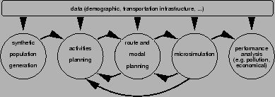
Simulation Modules

Traffic simulations for transportation planning typically consist of the following modules (Fig. 1):

• Population generation. Demographic data is disaggregated so that one obtains individual households and individual household members, with certain characteristics, such as a street address, car ownership, or household income (Beckman et al., 1996). - This module is not used for our current investigations but will be used in future.

• Activities generation. For each individual, a set of activities (home, going shopping, going to work, etc.) and activity locations for a day is generated (Vaughn et al., 1997; Bowman, 1998). - This module is not used in our current investigations but will be used in future.

• Modal and route choice. For each individual, the modes are selected and routes are generated that connect activities at different locations (see Sec. 2.1).

• Traffic micro-simulation. Up to here, all individuals have made plans about their behavior. The traffic micro-simulation executes all those plans simultaneously (see Sec. 2.2). In particular, we now obtain the result of interactions between the plans - for example congestion.

• Feedback. In addition, such an approach needs to make the modules consistent with each other (Sec. 2.3). For example, plans depend on congestion, but congestion depends on plans. A widely accepted method to resolve this is systematic relaxation - that is, make preliminary plans, run the traffic micro-simulation, adapt the plans, run the traffic micro-simulation again, etc., until consistency between modules is reached. The method is somewhat similar to the Frank-Wolfe-algorithm in static assignment, or in more general terms to a standard relaxation technique in numerical analysis.

This modularization has in fact been used for a long time; the main difference is that it is now feasible to make all modules completely microscopic, i.e. each traveler is individually represented in all modules.

Abbildung 1: TRANSIMS modules

Routing

Travelers/vehicles need to compute the sequence of links that they are taking through the network. A typical way to obtain such paths is to use a shortest path Dijkstra algorithm. This algorithm uses as input the individual link travel times plus the starting and ending point of a trip, and generates as output the fastest path.

It is relatively straightforward to make the costs (link travel times) time dependent, meaning that the algorithm can include the effect that congestion is time-dependent: Trips starting at one time of the day will encounter different delay patterns than trips starting at another time of the day. Link travel times are fed back from the micro-simulation in 15-min time bins, and the router finds the fastest route based on these 15-min time bins. Apart from relatively small and essential technical details, the implementation of such an algorithm is straightforward (Jacob et al., 1999). It is possible to include public transportation into the routing (Barrett et al., 1997); in our current work, we look at car traffic only.

Micro-Simulation

Our main micro-simulation is the queue simulation (Cetin and Nagel, in preparation; Gawron, 1998). The intent with this simulation is to keep travelers/vehicles microscopic and to have queue spillback, but apart from this to keep the simulation as simple as possible. This is similar in spirit to traffic simulations based on the smooth particle hydrodynamics approach, such as DYNEMO (Schwerdtfeger, 1987), DYNAMIT (its.mit.edu), or DYNASMART (Mahmassani et al., 1995).

In the queue simulation, streets are essentially represented as FIFO (first-in first-out) queues, with the additional restrictions that (1) vehicles have to remain for a certain time on the link, corresponding to free speed travel time; and that (2) there is a link storage capacity and once that is exhausted, no more vehicles can enter the link.

A major advantage of the queue simulation, besides its simplicity, is that it can run directly off the data typically available for transportation planning purposes. This is no longer true for more realistic micro-simulation, which need, for example, the number of lanes including pocket and weaving lanes, turn connectivities across intersections, or signal schedules.

Feedback

As mentioned above, plans (such as routes) and congestion need to be made consistent. This is achieved via a relaxation technique (Bottom, 2000; Kaufman et al., 1991; Nagel, 1994/95):

1. Initially, the system generates a set of routes based on free speed travel times.

2. The new routes are stored in a database, called the ``agent database'' (Raney and Nagel, 2002), so that the travelers (``agents'') may later associate the performance of the route to it, and may choose routes based on performance.

3. The traffic simulation is run with these routes.

4. Each agent measures the performance of his/her route based on the outcome of the simulation. ``Performance'' at present means the total travel time of the entire trip, with lower travel times meaning better performance. This information is stored for all the agents in the agent database, along with the route that was used.

5. 10% of the population requests new routes from the router, which bases them on the updated link travel times from the last traffic simulation. The new routes are then stored in the agent database.

6. Travelers who did not request new routes choose a previously tried route from the agent database by comparing performance values for the different routes. Specifically, they use a multinomial logit model
   
   $$p_i \propto e^{-\beta T_i}$$
   
   
   for the probability $p_i$ to select route $i$, where $T_i$ is the corresponding memorized travel time. $\beta$ was set heuristically to $1/(360 \hbox{sec})$ to obtain a fraction of about 10% non-optimal users.

7. This cycle (i.e. steps (3) through (6)) is run for 50 times; earlier investigations have shown that this is more than enough to reach relaxation (Rickert, 1998).

Note that this implies that routes are fixed during the traffic simulation and can only be changed between iterations. Work is under way to improve this situation, i.e. to allow online re-planning (Gloor, 2001).