Parallel Computing of the Queue Model

Abbildung 3: (a) The separation of flow capacity from intersection dynamics. (b) Test suite results for intersection dynamics. The curves show the number of discharging vehicles from two incoming links as explained in section 4.2. (c) Decomposition of the Switzerland street network. Each color corresponds to a different processor. (d) Communication between nodes in the boundaries: Node N1 needs to communicate with N2 and N3. Since N2 and N3 are on the same processor, they do not need to establish a communication between themselves.

[]

[]

[]

[]

Parallel Implementation

As was discussed above, the parallel target architecture for our transportation micro-simulation is a PC cluster. As also discussed, the suitable approach for this architecture is domain decomposition, i.e. to decompose the traffic network graph into several pieces, and to give each piece to a different CPU. Information exchange between CPUs is achieved via messages.

Next, one needs to decide where to split the graph, and how to achieve the message exchange. Both questions can only be answered with respect to a particular traffic model, which is why they were not discussed previously. Nevertheless, lessons learned here can be used for other models.

In general one wants to split as far away from the intersection as possible. This implies that one should split links in the middle, as for example TRANSIMS in fact does (30). However, for the queue model ``middle of the link'' does not make sense since there is no real representation of space. In consequence, one can either split at the downstream end, or at the upstream end of the link. The downstream end is undesirable because vehicles driving towards an intersection are more influenced by the intersection than vehicles driving away from an intersection. For that reason, in the queue simulation we split them right after the intersection (Fig. 3(d)).

With respect to message passing, this implies that a CPU that ``owns'' a split link reports, via a message, the number of empty spaces to the CPU which ``owns'' the intersection from which vehicles can enter the link. After this, the intersection update can be done in parallel for all intersections. Next, a CPU that ``owns'' an intersection reports, via a message, the vehicles that have moved to the CPUs which ``own'' the outgoing links. See Fig. 2(c) for pseudo-code of how this is implemented using message passing. In fact, Algorithm B and Algorithm C together give the whole pseudo-code for the queue model traffic logic. For efficiency reasons, all messages to the same CPU at the same time should be merged into a single message in order to incur the latency overhead only once.

Performance Issues

Once the precise implementation of the parallelization is known, it is possible to predict the parallel performance. This has been done in detail in Ref. (30). Since that reference refers to TRANSIMS instead of to the queue model, and since we also have results regarding Myrinet (www.myri.com), the most important aspects will be repeated here, with special focus towards the specific problems encountered in the current situation.

The execution time of a parallel program is defined as the total time elapsed from the time the first processor starts execution to the time the last processor completes the execution. During execution, on a PC cluster, each processor is either computing or communicating. Therefore,

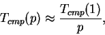
$$T(p) = T_{cmp}(p) + T_{cmm}(p) ,$$ (1)

where $T$ is the execution time, $p$ is the number of processors, $T_{cmp}$ is the computation time and $T_{cmm}$ is the communication time.

For traffic simulation, the time required for the computation, $T_{cmp}$ can be calculated roughly in terms of the run time of the computation on a single CPU divided by the number of processors. Thus,

$$T_{cmp}(p) \approx {T_{cmp}(1) \over p} ,$$ (2)

where $p$ is the number of CPUs. More exact formulas would also contain the overhead effects and unequal domain size effects (``load balancing'').

In deviation from Ref. (30), we now assume that the time for communication is well approximated by the latency only; this is in fact a good approximation for our system. Latency is incurred for each message that is sent. Since it is possible to pack all messages to the same processor into one message, one obtains

$$T_{lt} = N_{nb} t_{lt} ,$$

where $N_{nb}$ is the number of neighboring processors (i.e. the processors which are reached via common split links), and $t_{lt}$ is the latency per message.

The number of neighbors is zero at $p=1$, and goes, for contiguous domains, to an average of six for $p \to \infty$. An interpolating formula is

$$N_{nb}(p) = 2 (3 \sqrt{p} - 1) (\sqrt{p} - 1) / p ,$$ (3)

Latency of 100 Mbit Ethernet cards is about 0.5 ms; each processor sends messages twice per time step to all neighbors resulting in $\sim 12$ latency contributions or $6 ms$ per time step. In other words, the cluster can maximally do $1000/6=167$ time steps per second; in practice we find 174 with 64 CPUs, see Sec. 5.3. If the time step of a simulation is one second, then this is also the maximum real time ratio of the parallel simulation, i.e. the number which says how much faster than reality the computer is. Note that the limiting value does not depend on the problem size or on the speed of the algorithm; it is a limiting number for any parallel computation of a 2-dimensional system on a Beowulf cluster using Ethernet LAN.

The only way this number can be improved under the assumptions that we made is to use faster communication hardware. Gbit Ethernet hardware is faster, but standard driver implementations give away that advantage (25). In contrast, Myrinet (see www.myri.com) is a communication technology specifically designed for this situation. Interestingly, as we will see later, it will be possible to recoup the cost for a Myrinet network by being able to work with a smaller cluster.

Computational Performance

The parallel queue model is used as the traffic micro-simulation module within the project of a microscopic and activity-based simulation of all of Switzerland. In this paper, we only report computational performance results; validation results with respect to a real world scenario are reported elsewhere (37). Also note that our queue model is fully calibrated and validated in terms of free speed link travel times and link flow capacity, since these numbers are taken from the input files and implemented exactly. The same would be true for link storage capacity if those numbers were available. It was described earlier (Sec. 4.2) how intersection priorities are modeled, and how the implementation was verified.

The following performance numbers refer to the morning rush hour in a road network with 10564 nodes and 28624 links. Demand contains all car trips in Switzerland which start between 6:00AM and 9:00AM; this results in 991471 trips. The largest number of vehicles simultaneously in the simulation is 162464 vehicles at 8:00AM. This is also called the ``ch6-9'' scenario.

The most important plot is Fig. 4(a). It shows our newest (and fastest) computational real time ratio (RTR) numbers as a function of the number of CPUs. One notices that, with 64 CPUs, we reach an RTR of nearly 800. This means that we can simulate 24 hours of all car traffic in Switzerland less than two minutes! This performance is achieved with Myrinet communication hardware; with 100 Mbit Ethernet hardware, performance levels out at about 170 as predicted earlier. The plot also shows two different graphs for achieving the performance with single-CPU or with dual-CPU machines; one notices that there are differences but they are less important.

To the right of this, in Fig. 4(b), the corresponding speed-up curves are shown. In a log-log plot, the speed-up curve can be obtained from the RTR curve by a simple vertical shift; this vertical shift corresponds to a division by the RTR of the single-CPU version of the simulation, which is about 5 here. Speed-up curves put more emphasis on the efficiency of the implementation and less emphasis on the absolute speed. In our case, we reach super-linear speed-up, that is, the computational speed grows faster than the number of CPUs. This is due to the fact that for small numbers of CPUs, the simulation does not fit into computer memory, which is 1 GByte. For larger numbers of CPUs, some of the memory requirements get distributed across the CPUs, and so the memory requirement per CPU decreases.

Obviously, the speed-up curves show the same performance saturation for Ethernet as do the RTR curves. It should be noted that, while the level of saturation in the RTR curves is universal for this computer architecture and a one-second time step, for the speed-up curves this depends on the scenario size. Larger scenarios will reach higher speed-up, but saturate at the same RTR. For that reason, we consider the RTR number as more important than the speed-up.

The other curves in this figure show earlier performance numbers. Figs. 4(c) and 4(d) show the results of (). The curves are similar, but the performance is about 2-4 times slower. The reason is an improved implementation of the simulation logic in the newer results, in particular with respect to function inlining, etc.

Figs. 4(e) and 4(f) show the numbers that were presented last year at STRC (10). In spite of a smaller scenario, the RTR curves saturate at a much smaller value of 128. Worse, the speed-up did not get larger than 4, implying a very inefficient implementation. And indeed, in that implementation there was communication of every domain to every other domain, even if there was no relevant information to send. This means that number of messages per time step per CPU grows with $p$ (where $p$ is the number of CPUs), meaning that once the latency saturation sets in, performance decreases essentially as $\sim 1/p$. This is visible as convergence to a line with slope $-1$ in the log-log plots.

One could ask if a different domain decomposition might make a difference. It was already argued earlier that no difference is expected once the latency saturation sets in. Nevertheless, in earlier investigations we had found that there were some differences when using so-called multi-constraint partitioning in METIS when applied to the ``gotthard'' scenario (39). Yet, for the ch6-9 scenario, multi-constraint partitioning does not yield systematic improvement (not shown). Since this is consistent with the theoretical expectation that it should not yield a systematic improvement for spatially homogeneous scenarios, a further treatment of this is moved to the appendix.

It is interesting to compare two different hardware configurations:

• 64 single CPU machines using 100 Mbit LAN.

  Real time ratio 170.

  Cost approx $64 \times \$2 k = \$128 k$ for the machines plus approx $\$20 k$ for a full bandwidth switch, resulting in $\$148 k$ overall.

• 32 dual CPU machines using Myrinet.

  Real time ratio 770.

  Cost approx $32 \times \$4.5 k = \$144 k$, Myrinet included.

That is, the Myrinet set-up is not only considerably faster, but somewhat unexpectedly also cheaper. A Myrinet setup has the additional advantage that smaller scenarios than the one discussed will run even faster, whereas on the Ethernet cluster smaller scenarios will run with the same computational speed as the large scenarios.

Abbildung 4: (a) RTR and (b) Speedup curves of the ch6-9 scenario from Feb 2003, with the default domain decomposition approach. (c) RTR and (d) Speedup curves of the ch6-9 scenario from Nov 2002, with the default domain decomposition approach. (e) RTR and (f) Speedup curves of Gotthard scenario (fewer vehicles than in the 6-9 scenario) in March 2002. These results are from a non-optimized and unscalable version of queue simulator.

Feb 2003:

[] []

Nov 2002:

[] []

Mar 2002, also smaller scenario (``gotthard''):

[] []