THE AGENT DATABASE

Concept

In the above methods, all agents forgot their previous plans when new ones were created, on the assumption that the new ones were always better than the old ones. But, if the router is flawed, or not obtaining the proper information, this might not (always) be true. So, we now give the agents a memory of their past plans (also called decisions or strategies), and the outcome (performance of plans) of those decisions. We allow them to choose their new route plan based on the performance of the route plans in their memory. New, untested routes from the router iteration are given top priority, but if an agent has tried all of his/her plans before, then he/she chooses one by comparing their performance values. For an early version of this approach, see (48).

By giving the agents a memory, we must give them a way to select remembered routes. For a given plan -- as a whole -- we can find the total time taken to traverse the route. This will be a measure of the performance of the route. This is also called the ``score'' of the route strategy. Agents can compare scores of remembered routes, and choose one based only on performance information, without knowing anything else about the routes.

The idea here is that we do not need to fix the router to be perfect, as long as it generates reasonable routes most of the time. We can use the original router and travel time reporting strategies, and still get behavior that makes sense. An additional significant advantage is that with our system, other performance criteria besides travel time are easily implemented - one just needs to change the function that calculates the score. In order for that change to be meaningful, one needs a router that generates at least some routes which are ``good'' under the actual choice criterion that is implemented.

Implementation of the Agent Database

We introduce a database into the iteration framework to give the agents memory of their plans. Currently, this database is implemented in MySQL, an open-source relational database system (see www.mysql.org; SQL stands for ``Standard Query Language,'' and is the language used to exchange data with the database server). Each time the router generates a new plans file, those plans are added to the database, along with the identifying number of their corresponding agent, and the starting time of the plan. The database also stores, for each plan, the most recently measured travel time (score) made by the agent for that plan; and a flag that, when true, marks the plan as being the one used by its agent in the most recent micro-simulation. For new, untried plans generated by the router, the travel-time is considered to be zero, and the agent is forced to always choose that plan next. See Fig. 2(a) for an example of how the database stores information. At this stage, the database allows each agent to choose a plan (explained in more detail below), and updates the flags to reflect the new choices. These chosen plans are output to the micro-simulation for another run.

Figure 2: (a) Example tables in the agent database. The ``agent'' and ``plan_num'' fields are combined into the primary key for all three tables. The ``plan'' field of the plans table contains a text string consisting of link identifiers and other information that the router outputs.(b) Execution times of the linear-time feedback steps. (c) Execution times of the constant-time feedback steps. (d) Execution times of output-travel-times, with internal and external sorting. (e) Execution time contributions of all steps.

[]

plans table:
agent	plan_num	is_new	start_time	plan
1	1	0	25200	$<$text string 1$>$
1	2	1	25200	$<$text string 2$>$
2	1	0	25380	$<$text string 3$>$
$\vdots$	$\vdots$	$\vdots$	$\vdots$	$\vdots$

travel-times table:
agent	plan_num	travel_time
1	1	462
1	2	0
2	1	1047
$\vdots$	$\vdots$	$\vdots$

flags table:
agent	plan_num	flag
1	1	1
1	2	0
2	1	1
$\vdots$	$\vdots$	$\vdots$

[] [] [] []

After a simulation run is finished, its output is processed into link travel times for the router, and a file containing each agent's trip time. The latter is read into the database, where it is stored together with the corresponding route-plan. At this point, the database is ready for the next iteration, when the router will again generate a new set of plans that must be entered into the database.

How Plans Are Chosen Based on Performance

An important detail left out of the above explanation is how the performance (total travel-time) information is used by the agents to choose their plan for the next iteration. Each agent $a$ uses a logit model (16) to select option $i$:

where $T_{a,i}$ is the travel time.

The value of $\beta$ determines how likely it is that a ``non-best'' plan will be chosen. For the Gotthard scenario, we chose the value of $\beta$ so that about 90% of the agents would choose their best possible plan. The corresponding value of $\beta$ was .

Results of Agent Database on the Gotthard Scenario

Figure 1(e) shows the results of using the original feedback method from Sec. 6.1 plus the agent database, with plans selected as described above. As one can see, the freeway problem is avoided when the agents have memory of their plans, without any other changes in the router or in the travel time feedback. If the router starts putting too many agents on the side roads, some will eventually try out an old plan that used the freeway and find that it has a good performance, so will likely use that plan again. As long as they remember one or more plans that utilize the freeway, the agents can decide for themselves to use it, bypassing the side road choice of the router. Thus, the agent database gives an added flexibility and robustness to the system, so that even with a flawed router or feedback mechanism, the results come out satisfactorily. This value of $\beta$ we chose seemed to work well, but future work will likely need to explore the outcome of other values for this constant.

Computational Speed of the Agent Database

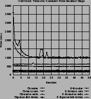
Figure 2 shows several graphs relating to the execution time as a function of iteration number for the important steps in the agent database feedback approach.

Besides for the Gotthard scenario, the agent database was also used for simulations of the 6-9 scenario, as explained in Sec. 5. Further information about this, including a comparison to static assignment results and to field data volume counts, are presented elsewhere (45). The computational performance results for that study are included here.

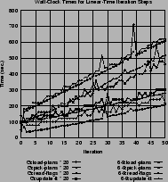
Figure 2(b) shows the execution time for those feedback steps that are linear in time based on their input size ( ${\mathbb{O}}(n)$). The number of plans in the database goes up by 10% each iteration, and the execution time of these operations is going up linearly with the iteration number (and thus the number of plans). So, we know that most of the database operations scale up (essentially) linearly. This graph also allows one to compare the results of the two test-cases, based on their problem size. The Gotthard scenario began with 50'000 plans while the 6-9 scenario began with 1'000'000. By multiplying the Gotthard execution times by 20, one can see those lines match with the 6-9 lines, further supporting linear complexity.

Figure 2(c) shows some other operations (such as parsing the events files) that do not have linear execution time, but mostly constant execution time ( ${\mathbb{O}}(1)$). These rely on the amount of data produced by the simulator, such as the number of events.

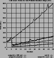
Figure 2(d) shows the execution time (for the 6-9 scenario only) of different versions of the output-travel-times operation, which requests the output of an agents' travel-time scores. In the ``old'' method, output-travel-times asked the database server to sort the information by the agent and plan number. This took a long time within the database (``output-tt w/DB sort''). This was improved significantly by asking the database for unsorted data and then sorting it externally (via the Unix ``sort'' command). The corresponding execution times for database output and for external sorting are ``output-tt unsorted'' and ``sort-tt''. Even when adding up those two time contributions (``output-tt + sort''), they are still significantly less than with the original approach.

Figure 2(e) summarizes the other three graphs by depicting the contribution of each operation to the total execution time of each iteration. In this figure, the results for the Gotthard scenario are omitted for clarity. The main point of this figure is that, excluding the microsimulation, the feedback process takes an average of about 2600 seconds (about 43 minutes) to execute for about 1 million agents.