Activities-based demand modeling

The problem with OD matrices is that they fix the travel demand once they have been derived. Thus, they fail to generate the effect of ``induced'' travel, which usually happens when one expands capacity. For example, a new freeway may induce people to make more trips, thus increasing overall travel. This means that one needs a demand generation method that is elastic with changing supply.

Activity-based methods attempt to achieve this by generating directly what people do during a day and where; transportation demand is thus derived by connecting activities at different locations (Fig. 21.1). There are at least two different methods to generate activities: econometric, and heuristic.

In principle, one can derive OD-matrices from activities, and many groups do this because it connects activity-based demand generation to existing models. This has, however, to be done with care since one loses important information. An important example of lost information are trip chains, where a person may go to work, may go shopping, and then home. If the person gets stuck on the way to shopping, the trip from shopping to home will take place later than anticipated; such effects do not get picked up in the OD matrix. Also, a universal reaction to changes in congestion seems to be to add or suppress intermediate stops at home, i.e. to replace home-work-home-shop-home by home-work-shop-home or vice versa. One would have to be careful to not suppress these possibilities when translating the trip chains into OD-matrices.

Econometric

[[I have discrete choice theory now in ``background'']]

[[dennoch k"onnte man fast alles hier lassen]]

[[need to sort out the $\beta_i$]]

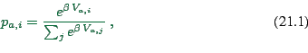
Econometric methods (15,38) are based on random utility theory, which will be explained in more detail in Chap. 29. An often-used choice model is the so-called logit model. If there are several options $i=1..N$, then the logit model predicts that the probability to select option $i$ is

$$p_{a,i} = \frac{e^{\beta \, V_{a,i}}}{\sum_j e^{\beta \, V_{a,j}}} \ ,$$

where $V_{a,i}$ is the utility (``score'') of option $i$ for a particular individual $a$, and $\beta$ is a parameter characterizing randomness. This equation was already used in Sec. 14.3, and the consequence of varying $\beta$ was discussed there.

[[have used $U$ in dep time choice. should use same notation as ben-akiva]]

For demand generation, one needs to make $V_{a,i}$ dependent on the attributes of the options, and on the properties of the individual under consideration. A typical assumption is to make this dependence linear:

$$V_i = \beta_1 \, x_{a,1} + ... + \beta_k \, x_{a,k} + \beta_{k+1} \, x_{i,k+1} + ... \ ,$$

[[now I have used $\beta$ twice, in slightly different meanings.]]

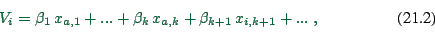
where the $x_{a,j}, j \le k$ are person attributes, and the $x_{i,j}, j > k$ are option attributes. For example, one could have

[[find one with bus, car, income]]

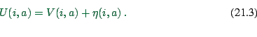
Utility theory assumes that the utility a person $i$ sees in a certain action $a$ is composed of a measurable and a non-measurable part:

$$U(i,a) = V(i,a) + \eta(i,a) \ .$$

Under a variety of assumptions, e.g. that $\eta$ is a random variable and follows a certain distribution, this leads to an equation for the probability to choose action $a$.

An often-used discrete choice model is the so-called logit model. Its main assumptions are:

• Individuals and actions are characterized by certain attributes, that is, two individuals with the same attributes will be modeled by the same equation. This also means that $i$ and $a$ are replaced by a vector of attributes, $\vec x_{i,a}$.

• The measurable part of the utilities, $V$, is a linear function of the attributes, i.e. $V = \vec \beta \cdot \vec x$.

• The random variables $\eta$ do not depend on the attributes $\vec x_{i,a}$, and they are Gumbel distributed, i.e. the generating function is
  
  $$F(\eta) = \exp[ - e^{- \mu \, (\eta - \gamma) } ] \ ,$$
  
  
  which results in the distribution
  
  $$f(\eta) = \mu \, e^{- \mu \, (\eta - \gamma) } \, \exp[ - e^{- \mu \, (\eta - \gamma)} ]$$
  
  
  $\gamma$ is a location parameter, and $\mu$ is a positive scale parameter. This distribution is somewhat similar to an asymmetric version of the normal distribution; its main advantage is that it leads to a closed form solution of the choice model.

With a logit model, the probability to choose the bus in a decision between bus and car could look as follows:

$$P(bus) = {\exp[ - \beta_b \, t_b ] \over \exp[ - \beta_b \, t_b ] + \exp[ - \beta_c \, t_c ] } \ .$$ (21.1)

$t_b$ and $t_c$ are the respective travel times the trip would take by bus or by car. $\beta_b$ and $\beta_c$ are factors which weigh time in the bus vs. time in the car, i.e. they are ``values of time''. For example, one could say that time in the bus is more productive than in the car because one can read, resulting in $\beta_b > \beta_c$. However, usually the car is faster, compensating for this effect. - Note that Eq. 21.6 has the same functional form as a Boltzmann distribution.

The $\beta_b$ and $\beta_c$ are estimated from surveys, for example via maximum likelihood methods. A sample of the population with different car and bus travel times is asked about their choices, and the $\beta_x$ are determined such that the probability according to Eq. 21.6 to re-generate the survey is maximized.

For applications inside a transportation simulation, this becomes a lot more complicated. An implementation for Portland/Oregon (17) determines activity patterns (for example home-work-home or home-work-shop-home), activity timing, activity locations, mode choice, etc. As long as one wants to treat all alternatives simultaneously, this has the problem that the number of coefficients grows exponentially. For example, if one has five activities patterns, and three modes of transportation, this means 15 different choices and thus 15 parameters. If however one does not treat the alternatives simultaneously, one can make mistakes: For example, a person could have a strong preference for a pattern home-work-home-shop-home when averaged over all possible circumstances, but may prefer home-work-shop-home when really good bus service is available. When choosing first the pattern and then the transportation mode, this information gets misrepresented.

Heuristic methods

The econometric method has a solid theoretical foundation, and it is currently the only method that is functional for transportation simulations. However, sometimes it seems like it does not really represent how people behave. The discrete choice method pretends that people calculate utilities for all possible alternatives and then choose the alternative with the highest utility. (Remember that the randomization just comes in because of ``unobserved attributes''.) However, people do not do this. For example, they may discard an activity pattern home-shop-work-home right away without calculating the utilities of all possible constellations.

Heuristic methods attempt to better represent such human planning processes. For example, research shows that humans make their planning decisions on many time scales simultaneously (37). The time for work is usually alloted way in advance, shopping may be planned a day in advance, and then the whole schedule may be changed short-term because the child gets sick. Prototypes for such models exist, but they seem currently far away from being operational in any meaningful way.

It should be noted that heuristic and econometric methods can be combined. For example, one could use a heuristic method to determine which decisions are made how far in advance, and use an econometric method to make the actual decision. Or the econometric method could calculate the probability for each activities pattern, the heuristic method could decide to retain the two most important patterns, the econometric method than could calculate the utilities for these two patterns for all mode and time combinations, etc.

Summary of activities-based methods

Activities-based demand generation models are a promising method for transportation simulation. Some implementations of these methods have reached the state where they can be used for actual applications (18). However, so far there are only very few results about coupling these methods together with transportation micro-simulations, as intended with the transportation planning simulation packages described in this article. The only functional system that we are aware of uses a very simple method of demand generation; it is described in the appendix. But we are optimistic that research in the next couple of years will expand the boundaries in these areas enormously.