Knowledge of agents should be private, i.e. each agent should have a different set of knowledge items. For example, people typically only know a relatively small subset of the street network (``mental map''), and they have different knowledge and perception of congestion. This suggests the use of Complex Adaptive Systems methods (e.g. (56)). Here, each agent has a set of strategies from which to choose, and indicators of past performance for these strategies. The agent normally choses a well-performing strategy. From time to time, the agent choses one of the other strategies, to check if its performance is still bad, or replaces a bad strategy by a new one.
This approach divides the problem into three parts (see also (14)):
As usual, the challenge is to balance exploration (including generation) and exploitation. This is particularly problematic here because of the co-evolution aspect: If too many agents do exploration, then the system performance is not representative of a ``normal'' performance, and the exploring agents do not learn anything at all. If, however, they explore too little, the system will relax too slowly (cf. ``run 4'' and ``run 5'' in Fig. 31.1). We have good experiences with the following scheme:
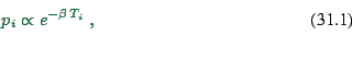 |
(31.1) |
A major advantage of this approach is that it becomes more robust against artifacts of the router: if an implausible route is generated, the simulation as a whole will fall back on a more plausible route generated earlier. Fig. 31.2 shows an example. The scenario is the same as in Fig. 2.4 of Chap. 2; the location is slightly north of the final destination of all trips. We see snapshots of two relaxed scenarios. The left plot was generated with a standard relaxation method as described in the previous section, i.e. where individual travelers have no memory of previous routes and their performance. The right plot in contrast was obtained from a relaxation method which uses exactly the same router but which uses an agent data base, i.e. it retains memory of old options. In the left plot, we see that many vehicles are jammed up on the side roads while the freeway is nearly empty, which is clearly implausible; in the right plot, we see that at the same point in time, the side roads are empty while the freeway is just emptying out - as it should be.
The reason for this behavior is that the router miscalculates at which time it expects travelers to be at certain locations - specifically, it expects travelers to be much earlier at the location shown in the plot. In consequence, the router ``thinks'' that the freeway is heavily congested and thus suggests the side road as an alternative. Without an agent data base, the method forces the travelers to use this route; with an agent data base, agents discover that it is faster to use the freeway.
This means that now the true challenge is not to generate exactly the correct routes, but to generate a set of routes which is a superset of the correct ones (14). Bad routes will be weeded out via the performance evaluation method. For more details see (). Other implementations of partial aspects are (124,116,115,51).
The way we have explained it, each individual needs computational
memory to store his/her plan or plans. The memory requirements for
this are of the order of
![]() , where
, where ![]() is the number of
people in the simulation,
is the number of
people in the simulation, ![]() is the number of trips a person
takes per day,
is the number of trips a person
takes per day, ![]() is the average number of links between
starting point and destination, and
is the average number of links between
starting point and destination, and ![]() is the number of
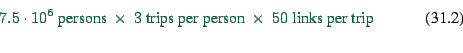
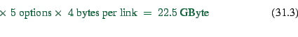
options remembered per agent. For example, for a 24-hour simulation
of all traffic in Switzerland, we have
is the number of
options remembered per agent. For example, for a 24-hour simulation
of all traffic in Switzerland, we have
![]() ,
,
![]() ,
,
![]() , and
, and
![]() , which results in
, which results in
 |
(31.2) |
 |
(31.3) |
Since this is a large storage requirement, many approaches do not
store plans in this way. They store instead the shortest path for
each origin-destination combination. This becomes affordable since
one can organize this information in trees anchored at each possible
destination. Each intersections has a ``signpost'' which gives, for
each destination, the right direction; a plan is thus given by knowing
the destination and following the ``signs'' at each intersection. The
memory requirements for this are of the order of
![]() , where
, where ![]() is the number
of nodes of our network, and
is the number
of nodes of our network, and
![]() is the number of
possible destinations.
is the number of
possible destinations. ![]() is again the number of options,
but note that these are options per destination, so different
agents traveling to the same destination cannot have more than
is again the number of options,
but note that these are options per destination, so different
agents traveling to the same destination cannot have more than
![]() different options between them.
different options between them.
Traditionally, transportation simulations use of
the order of 1000 destination zones, and networks with of the
order of 10000 nodes, which results in a memory requirement of
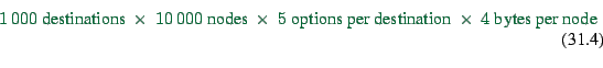 |
(31.4) |
The problem with this second approach is that it explodes with more
realistic representations. For example, for our simulations we
usually replace the traditional destinations zones by the links, i.e.
each of typically 30000 links is a possible destination. In
addition, we need the information time-dependent. If we assume that
we have 15-min time slices, this results in a little less than
100 time slices for a full day.
The memory requirements for the second method now become
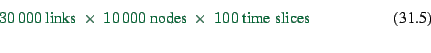 |
(31.5) |
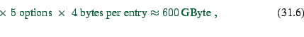 |
(31.6) |
![\includegraphics[width=0.7\hsize]{gz/individualization.eps.gz}](img733.png)
|