We like to interpret our agents and in consequence the whole system as ``learning''. It is however difficult to exactly define the term ``learning''; for example, what is the difference between learning and adaptation? Similarly, it is difficult to formally state the goal of our agents. In the traditional interpretation of economics, reflected in Wardrop's first principle in Chap. 28, agents try to reach a Nash equilibrium, meaning that they are not able to improve by unilaterally changing their strategy. This is however well-defined only within relatively confined formal frameworks and difficult to apply both in complex simulations such as ours and in the real world.
As a first step, it is useful to treat our learning dynamics as a time-discrete dynamical system, and ignore all interpretation. The learning system iterates from one day (period) to the next; a state is all information the system possesses or generates during that day, including agent memory and the trajectory of the simulation through one day; an iteration is the update from one day to the next (Fig. 31.3, although that figure excludes agent memory).
Let us, in order to have some formal symbols at our disposal, denote
the state of the system on day ![]() as
as ![]() , and let us denote the
operator which maps the system from day
, and let us denote the
operator which maps the system from day ![]() to day
to day ![]() as
as ![]() :
:
 |
(31.7) |
[[bottom multi-step iteration?]]
In such a dynamical system, one can search for properties like fixed points, steady state probabilities, multiple basins of attraction, strange attractors, etc. The assumption behind all these concepts is that the system starts out with some arbitrary state, given by the experimentators, but from there on goes to some other state where it will remain.
[[need fig]]
We will assume that our simulations are Markovian, meaning that
the state at period ![]() depends on information from the period
depends on information from the period ![]() only. If some knowledge about earlier history is involved, then we
assume that this is made part of the state at period
only. If some knowledge about earlier history is involved, then we
assume that this is made part of the state at period ![]() . An example
for this are the scores of the agents, which contain knowledge from
earlier periods. We also assume that the knowledge space of the
agents does not infinitely increase, i.e. there is a limit on how
many options they remember, and a limit on how much information about
the past they remember. For example, when trying the same option
several times, the information could be subsumed into a moving
average.
. An example
for this are the scores of the agents, which contain knowledge from
earlier periods. We also assume that the knowledge space of the
agents does not infinitely increase, i.e. there is a limit on how
many options they remember, and a limit on how much information about
the past they remember. For example, when trying the same option
several times, the information could be subsumed into a moving
average.
Next, we differentiate between deterministic and stochastic systems. Clearly, our transportation simulations are stochastic. Nevertheless, the theory of deterministic dynamic systems provides useful insights and often a language to describe what we observe in our systems.
![\includegraphics[width=0.8\hsize]{mapping-fig.eps}](img738.png)
|
It is often of interest to describe the behavior of a system for long times. The following are examples of what can happen. The phenomena do not exclude each other:
Fixed point: A state which repeats itself:
 |
(31.8) |
Periodic behavior: A cycle which repeats itself:
 |
(31.9) |
Chaotic behavior: Complicated movement, seemingly without rules or structure. Slightly different initial conditions eventually lead to total divergence of the trajectories.
Attractor: A sub-region in state space where the system goes to. Attractors can for example be fixed points, periodic or chaotic.
A basin of attraction is the region of state space which leads to a specific attractor.
Ergodic behavior: The long time trajectory comes arbitrarily close to every point in state space.
Note, for example, that static assignment (Chap. 28) has, under certain conditions, only one optimum. That means that plausible learning dynamics for the static assignment problem have exactly one basin of attraction, and they all lead to the same fixed point solution. This lets us speculate that the result of Sec. 31.2, i.e. that many learning algorithms seem to lead to the same steady state behavior, is caused by structural aspects of the problem, which carry over from static assignment to the simulation variant.
In stochastic systems, a state at period ![]() can typically go to more
than one state at period
can typically go to more
than one state at period ![]() . This means that in general the notion
of a fixed point does not make sense, and needs to be replaced by a
time-invariant probability distribution. That is, one looks at
the probability
. This means that in general the notion
of a fixed point does not make sense, and needs to be replaced by a
time-invariant probability distribution. That is, one looks at
the probability ![]() for each state
for each state ![]() , and how it behaves under
our update. Such a probability distribution is time-invariant if
, and how it behaves under
our update. Such a probability distribution is time-invariant if
 |
(31.10) |
Often the words ``in equilibrium'', ``steady-state'', or ``stationary'' are used instead of time-invariant probability distribution.
Again, very little can be said in general about when a system reaches equilibrium. Two conditions which when simultaneously fulfilled lead to convergence to equilibrium are ``ergodic'' and ``mixing'':
Ergodic: A system is ergodic if the system can get arbitrarily close to each state from every other state, possibly via a chain of intermediate states.
[[This definition does not satisfy detailed balance. But I think it is correct. Check!!]]
Mixing: Any initial distribution in state space will spread out and eventually cover the whole state space.
[[check. In particular, in det Hamiltonian systems, initial phase space vol does not increase, it only fuzzyfies. In stoch systems, this should be different. ]]
What this means intuitively is: Let us start with infinitely many
replicas of the same state ![]() but with different random seeds.
Being in the same state means that
but with different random seeds.
Being in the same state means that
![]() . If the
system is mixing, then after infinite time the probability to find a
randomly picked system in state
. If the
system is mixing, then after infinite time the probability to find a
randomly picked system in state ![]() is
is ![]() , i.e. the steady
state density.
, i.e. the steady
state density.
In simulation practice, these characterizations are close to useless. Even when a system is both ergodic and mixing, it can display broken ergodicity, meaning that it can remain in a part of the state space for arbitrarily long time (93). For those who happen to know this, a finite size Ising model below the critical temperature is an example. Another example is a stochastic search algorithm being stuck in a local optimum.
[[fig]]
To make matters worse, we are not necessarily interested in the steady state learning solution, but possibly in the transients. For example, when an important bridge is closed for construction, prediction of the first days after the closure may be as important as prediction of the long term behavior. Worse, aspects such as land use or the housing market in practice probably never reach the steady state.
To put this into context, consider a simple ordinary differential
equation,
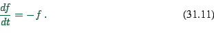 |
(31.11) |
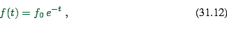 |
(31.12) |