Computational Aspects

Computational performance of the mobility simulation

It is possible to make the mobility simulation parallel, i.e. to give different pieces of it to different CPUs (Central Processing Units). One good option is to do this via domain decomposition; that is, the geographical area is decomposed into domains, and each CPU computes traffic within that domain. These domains need to exchange information at their borders, which can be achieved by messages. For messages, existing message passing software such as MPI (Message Passing Interface, www.mcs.anl.gov/mpi/) or PVM (Parallel Virtual Machine, www.epm.ornl.gov/pvm) can be used.

In this situation, simulation time per time step is a sum of the time spent on computation and the time spent on communication,

$$T(p) = T_{cmp}(p) + T_{cmm}(p) \ ,$$

where $p$ is the number of CPUs. For the purposes of an intuitive understanding, let us assume that

$$T_{cmp}(p) \approx \frac{T_1}{p} \ ,$$

i.e. that there is a true distribution of work. $T_1$ is the time a single CPU needs. For the communication, it turns out that the main component is the latency $t_{lat}$ of the communication. Latency refers to the amount of time that is necessary to prepare a message before it can be sent away. Most of that time is caused by the hardware, such as Ethernet, and the corresponding Internet protocols, such as TCP/IP. For 100 Mbit Ethernet, this latency time is of the order of $0.5~msec$. Since in two-dimensional systems each domain has in the average six neighbors, and we need two messages per time step, communication time can be approximated as

$$T_{cmm}(p) \approx 12 \, t_{lat} \ .$$

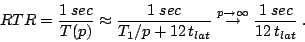
Overall, this results in

$$T(p) \approx \frac{T_1}{p} + 12 \, t_{lat} \ .$$

Let us define the real time ratio as how much faster than reality the simulation is. If we assume that one simulation time step corresponds to one second, then we obtain

$$RTR = \frac{1~sec}{T(p)} \approx \frac{1~sec}{T_1/p + 12 \,... ...} \stackrel{p \to \infty}{\to} \frac{1~sec}{12 \, t_{lat}} \ .$$ (2)

For 100 Mbit Ethernet, $t_{lat} \approx 0.5~msec$, and therefore $RTR \to 167$ for $p \to \infty$. In words:

This statement is independent of the problem size or of the specific model, it only depends on the fact that a simulation time-step corresponds to one second.

The actual performance measurements in Fig. 5(a) from our implementation (dots) demonstrate that these concerns are justified. The line is a fit to those performance measurements, based on the mathematical form of Eq. (2). The results of Fig. 5 refer to runs of the Switzerland 6-9 scenario as explained above. Only with a faster communication hardware, Myrinet (www.myri.com), this bottleneck can be overcome and much faster simulations can be achieved. Our best performance currently is an RTR of nearly 800. This means that a whole day of all car traffic in Switzerland, which has about 7 mio inhabitants, can be simulated in less than 2 minutes. This makes now large scale learning studies possible, although it should be noted that these performance numbers are obtained without taking data input and output into account.

Fig. 5(b) also shows the speedup for the same runs. Speedup is defined as the performance ratio between a multi-CPU and a single-CPU run:

$$Speedup(p) = \frac{T(p)}{T_1} \ .$$

As one can see in the plots, speedup is obtained by shifting the RTR curve vertically; the amount of shifting is given by the RTR of the single-CPU run. As one sees, our fastest simulation is, on 64 CPUs, about 200 times faster than the single-CPU simulation. This so-called super-linear speedup is caused by the fact that the scenario is too large to fit comfortably into a single-CPU machine and thus causes slow memory paging there. Without further information, speedup curves cannot be used to understand real time limitations on the computation, which is important for ITS applications. - More information can be found in Cetin and Nagel (15).

Figure 5: (a) RTR and (b) Speedup curves of the ch6-9 scenario from Feb 2003, with the default domain decomposition approach. Dots refer to actual computational benchmarks; the solid line is based on the theory explained in the text.

Feb 2003:

[] []

Computational performance of a full iteration

Figure 6 depicts the cumulative contributions of the major steps in the feedback system to the total execution time of each iteration. The left figure shows the implementation of the feedback mechanism with MySQL (www.mysql.org), a file-based database. As explained in Sec. 4, the agent database keeps track of agent strategies and their scores. The right figure shows an implementation where all relevant data (i.e. strategies) are permanently kept in computer memory. Rather than using slower scripting languages for each step in the iteration (48), the new implementation is written in C++ and combines all operations into one program. The figure shows computational performance results for the scenario described in Sec. 5; the contributions shown in the figure are:

1. Strategy Generation adds a new strategy for 10% of the agents into the database. Once the network data has relaxed, this step takes about the same amount of time in each iteration.

2. Strategy Selection, where the other 90% of the agents select a strategy from the database. In the left figure, the execution time for this step scales approximately linearly with the total number of strategies stored in the agent database. Thus, it takes longer to execute with each iteration. In the right figure it takes essentially the same amount of time in each iteration.

3. Mobility Simulation, where the agents interact. This again relaxes to a consistent amount of time, though takes longer in earlier iterations when there is more congestion to deal with. In the left figure, this step ends up taking about 15 minutes while in the right it ends up taking only about 10 minutes. This is due to an improvement in the mobility simuation speed between trials, and has nothing to do with the agent database.

4. Score Update, where the agents update the performance scores of their executed strategy from the output of the mobility simulation. The execution time for this operation is fairly constant in each iteration, since it depends on the number of events produced by the simulation (see Sec. 2). This number is proportional to the number of agents and the length of their routes; it does not change very much from one iteration to the next. In the left figure, this operation takes about 20 minutes while in the right figure it takes about 10 minutes.

More details about the database implementation and execution times can be found in Raney and Nagel (48).

One can see that in the left figure, on average each iteration takes about an hour to execute, with the feedback system, with strategy-related steps totaling about 45 minutes of that time. The overall result is that we can run a metropolitan scenario with 1 million agents, including 50 learning iterations, in about two days.

For the right figure, the total time is cut in half, with about 20 minutes spent on strategy-related steps.

Figure 6: Cumulative Execution Time Contributions of Major Iteration Steps LEFT: File-based database implementation. RIGHT: The new implementation, which keeps all agent information in computer memory, and which also uses a faster mobility simulation.