In the last section, we explained how the street network is partitioned into domains that can be loaded onto different CPUs. In order to be efficient, the loads on different CPUs should be as similar as possible. These loads do however depend on the actual vehicle traffic in the respective domains. Since we are doing iterations, we are running similar traffic scenarios over and over again. We use this feature for an adaptive load balancing: During run time we collect the execution time of each link and each intersection (node). The statistics are output to file. For the next run of the micro-simulation, the file is fed back to the partitioning algorithm. In that iteration, instead of using the link lengths as load estimate, the actual execution times are used as distribution criterion. Fig. 9 shows the new domains after such a feedback (compare to Fig. 5).
To verify the impact of this approach we monitored the execution times per time-step throughout the simulation period. Figure 10 depicts the results of one of the iteration series. For iteration 1, the load balancer uses the link lengths as criterion. The execution times are low until congestion appears around 7:30 am. Then, the execution times increase fivefold from 0.04 sec to 0.2 sec. In iteration 2 the execution times are almost independent of the simulation time. Note that due to the equilibration, the execution times for early simulation hours increase from 0.04 sec to 0.06 sec, but this effect is more than compensated later on.
The figure also contains plots for later iterations (11, 15, 20, and 40). The improvement of execution times is mainly due to the route adaptation process: congestion is reduced and the average vehicle density is lower. On the machine sizes where we have tried it (up to 16 CPUs), adaptive load balancing led to performance improvements up to a factor of 1.8. It should become more important for larger numbers of CPUs since load imbalances have a stronger effect there.
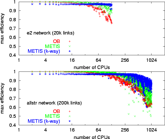
Figure 9: Partitioning after adaptive load balancing. Compare to
Fig. 5.
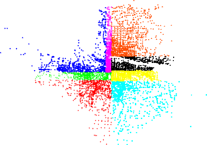
Figure 10: Execution times with external load feedback. These results were
obtained during the Dallas case
study [4, 34].