Performance prediction for the TRANSIMS micro-simulation

 

It is possible to systematically predict the performance of parallel micro-simulations (e.g. [19, 26]). For this, several assumptions about the computer architecture need to be made. In the following, we demonstrate the derivation of such predictive equations for coupled workstations and for parallel supercomputers.

The method for this is to systematically calculate the wall clock time for one time step of the micro-simulation. We start by assuming that the time for one time step has contributions from computation, $T$_cmp, and from communication, $T$_cmm. If these do not overlap, as is reasonable to assume for coupled workstations, we have

$T(p)\; =\; T$_cmp(p) + T_cmm(p) ,

where $p$ is the number of CPUs.

Time for computation is assumed to follow

$T$_cmp(p) = T₁ p ( 1 + f_ovr(p) + f_dmn(p) ) .

Here, $T$₁ is the time of the same code on one CPU (assuming a problem size that fits on available computer memory); $p$ is the number of CPUs; $f$_ovr includes overhead effects (for example, split links need to be administered by both CPUs); $f$_dmn = 1/e_dmn - 1 includes the effect of unequal domain sizes discussed in Sec. 6.

Time for communication typically has two contributions: Latency and bandwidth. Latency is the time necessary to initiate the communication, and in consequence it is independent of the message size. Bandwidth describes the number of bytes that can be communicated per second. So the time for one message is

$T$_msg = T_lt + S_msg b ,

where $T$_lt is the latency, $S$_msg, is the message size, and $b$ is the bandwidth.

However, for many of today's computer architectures, bandwidth is given by at least two contributions: node bandwidth, and network bandwidth. Node bandwidth is the bandwidth of the connection from the CPU to the network. If two computers communicate with each other, this is the maximum bandwidth they can reach. For that reason, this is sometimes also called the ``point-to-point'' bandwidth.

The network bandwidth is given by the technology and topology of the network. Typical technologies are 10 Mbit Ethernet, 100 Mbit Ethernet, FDDI, etc. Typical topologies are bus topologies, switched topologies, two-dimensional topologies (e.g. grid/torus), hypercube topologies, etc. A traditional Local Area Network (LAN) uses 10 Mbit Ethernet, and it has a shared bus topology. In a shared bus topology, all communication goes over the same medium; that is, if several pairs of computers communicate with each other, they have to share the bandwidth.

For example, in our 100 Mbit FDDI network (i.e. a network bandwidth of $b$_net = 100 Mbit) at Los Alamos National Laboratory, we found node bandwidths of about $b$_nd = 40 Mbit. That means that two pairs of computers could communicate at full node bandwidth, i.e. using 80 of the 100 Mbit/sec, while three or more pairs were limited by the network bandwidth. For example, five pairs of computers could maximally get $100/5\; =\; 20$ Mbit/sec each.

A switched topology is similar to a bus topology, except that the network bandwidth is given by the backplane of the switch. Often, the backplane bandwidth is high enough to have all nodes communicate with each other at full node bandwidth, and for practical purposes one can thus neglect the network bandwidth effect for switched networks.

If computers become massively parallel, switches with enough backplane bandwidth become too expensive. As a compromise, such supercomputers usually use a communications topology where communication to ``nearby'' nodes can be done at full node bandwidth, whereas global communication suffers some performance degradation. Since we partition our traffic simulations in a way that communication is local, we can assume that we do communication with full node bandwidth on a supercomputer. That is, on a parallel supercomputer, we can neglect the contribution coming from the $b$_net-term. This assumes, however, that the allocation of street network partitions to computational nodes is done in some intelligent way which maintains locality.

As a result of this discussion, we assume that the communication time per time step is

$T$_cmm(p) = N_sub ( n_nb(p)   T_lt + N_spl(p) p S_bnd b_nd + N_spl(p)   S_bnd b_net ) ,

which will be explained in the following paragraphs. $N$_sub is the number of sub-time-steps. As discussed in Sec. 4, we do two boundary exchanges per time step, thus $N$_sub=2 for the 1999 TRANSIMS micro-simulation implementation.

$n$_nb is the number of neighbor domains each CPU talks to. All information which goes to the same CPU is collected and sent as a single message, thus incurring the latency only once per neighbor domain. For $p=1$, $n$_nb is zero since there is no other domain to communicate with. For $p=2$, it is one. For and assuming that domains are always connected, Euler's theorem for planar graphs says that the average number of neighbors cannot become more than six. Based on a simple geometric argument, we use

$n$_nb(p) = 2   (3 p - 1)   (p - 1) / p ,

which correctly has $n$_nb(1) = 0 and $n$_nb →6 for . Note that the METIS library for graph partitioning (Sec. 6) does not necessarily generate connected partitions, making this potentially more complicated.

$T$_lt is the latency (or start-up time) of each message. $T$_lt between 0.5 and 2 milliseconds are typical values for PVM on a LAN [34, 11].

Next are the terms that describe our two bandwidth effects. $N$_spl(p) is the number of split links in the whole simulation; this was already discussed in Sec. 6 (see Fig. 6). Accordingly, $N$_spl(p)/p is the number of split links per computational node. $S$_bnd is the size of the message per split link. $b$_nd and $b$_net are the node and network bandwidths, as discussed above.

In consequence, the combined time for one time step is

$T(p)\; =\; T$₁ p ( 1 + f_ovr(p) + f_dmn(p) ) +

$N$_sub {( n_nb(p)   T_lt + N_spl(p) p S_bnd b_nd + N_spl(p)   S_bnd b_net } .

According to what we have discussed above, for the number of neighbors scales as $n$_nb const and the number of split links in the simulation scales as $N$_spl p. In consequence for $f$_ovr and $f$_dmn small enough, we have:

• for a shared or bus topology, $b$_net is relatively small and constant, and thus

  $T(p)\; 1\; p\; +\; 1\; +\; 1p+p\to p;$

• for a switched or a parallel supercomputer topology, we assume $b$_net = &inf; and obtain

  $T(p)\; 1\; p\; +\; 1\; +\; 1p\to 1\; .$

Thus, in a shared topology, adding CPUs will eventually increase the simulation time, thus making the simulation slower. In a non-shared topology, adding CPUs will eventually not make the simulation any faster, but at least it will not be detrimental to computational speed. The dominant term in a shared topology for is the network bandwidth; the dominant term in a non-shared topology is the latency.

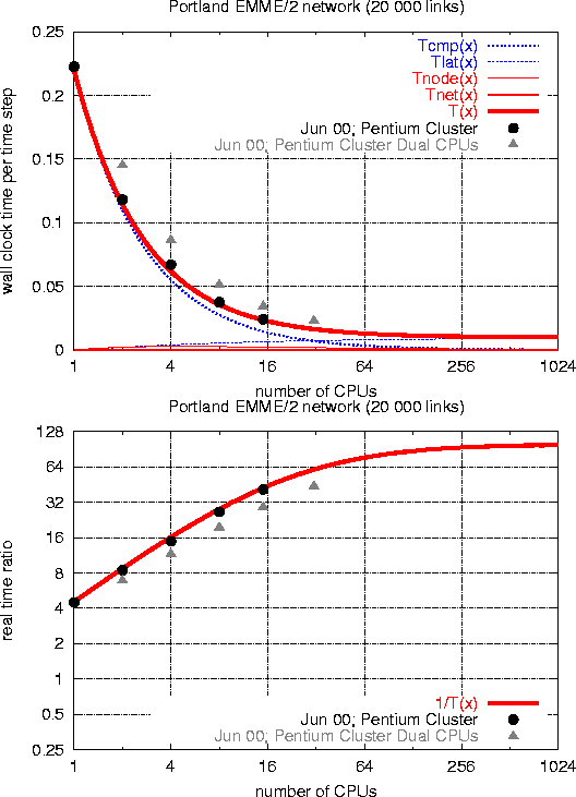
The curves in Fig. 11 are results from this prediction for a switched 100 Mbit Ethernet LAN; dots and crosses show actual performance results. The top graph shows the time for one time step, i.e. $T(p)$, and the individual contributions to this value. The bottom graph shows the real time ratio (RTR)

$rtr(p)\; :=\; \Delta t\; T(p)\; =\; 1 sec\; T(p)\; ,$

which says how much faster than reality the simulation is running. $\Delta t$ is the duration a simulation time step, which is $1 sec$ in TRANSIMS-1999. The values of the free parameters are:

• Hardware-dependent parameters. We assume that the switch has enough bandwidth so that the effect of $b$_net is negligeable. Other hardware parameters are $T$_lt = 0.8 ms and $b$_nd = 50 Mbit/s.
• Implementation-dependent parameters. The number of message exchanges per time step is $N$_sub=2.
• Scenario-dependent parameters. Except when noted, our performance predictions and measurements refer to the Portland 20024 links network. We use, for the number of split links, $N$_spl(p) = 140 p^0.59 - 140, as explained in Sec. 6.
• Other Parameters. The message size depends on the plans format (which depends on the software design and implementation), on the typical number of links in a plan, and on the frequency per link of vehicles migrating from one CPU to another. We use $S$_bnd = 200 Bytes. This is an average number; it includes all the information that needs to be sent when a vehicle migrates from one CPU to another. The new TRANSIMS multi-modal plans format easily has 200 entries per driver and trip, resulting in 800 bytes of information just for the plan. In addition, there is information about the vehicle (ID, speed, maximum acceleration, etc.); however, not in every time step a vehicle is migrated across a boundary on every split link. In principle it is however possible to compress the plans information, so improvements are possible here in the future. Also, we have not explicitely modelled simulation output, which is indeed a performance issue on Beowulf clusters.

These parameters were obtained in the following way: First, we obtained plausible values via systematic communication tests using messages similar to the ones used in the actual simulation [34]. Then, we ran the simulation without any vehicles (see below) and adapted our values accordingly. Running the simulation without vehicles means that we have a much better control of $S$_bnd. In practice, the main result of this step was to set $t$_lat to 0.8 msec, which is plausible when compared to the hardware value of 0.5 msec. Last, we ran the simulations with vehicles and adjusted $S$_bnd to fit the data. -- In consequence, for the switched 100 Mbit Ethernet configurations, within the data range our curves are model fits to the data. Outside the data range and for other configurations, the curves are model-based predictions.

The plot (Fig. 11) shows that even something as relatively profane as a combination of regular Pentium CPUs using a switched 100Mbit Ethernet technology is quite capable in reaching good computational speeds. For example, with 16 CPUs the simulation runs 40 times faster than real time; the simulation of a 24 hour time period would thus take 0.6 hours. These numbers refer, as said above, to the Portland 20024 links network. Included in the plot (black dots) are measurements with a compute cluster that corresponds to this architecture. The triangles with lower performance for the same number of CPUs come from using dual instead of single CPUs on the computational nodes. Note that the curve levels out at about forty times faster than real time, no matter what the number of CPUs. As one can see in the top figure, the reason is the latency term, which eventually consumes nearly all the time for a time step. This is one of the important elements where parallel supercomputers are different: For example the Cray T3D has a more than a factor of ten lower latency under PVM [11].

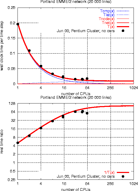
As mentioned above, we also ran the same simulation without any vehicles. In the TRANSIMS-1999 implementation, the simulation sends the contents of each CA boundary region to the neighboring CPU even when the boundary region is empty. Without compression, this is five integers for five sites, times the number of lanes, resulting in about 40 bytes per split edge, which is considerably less than the 800 bytes from above. The results are shown in Fig. 12. Shown are the computing times with 1 to 15 single-CPU slaves, and the corresponding real time ratio. Clearly, we reach better speed-up without vehicles than with vehicles (compare to Fig. 11). Interestingly, this does not matter for the maximum computational speed that can be reached with this architecture: Both with and without vehicles, the maximum real time ratio is about 80; it is simply reached with a higher number of CPUs for the simulation with vehicles. The reason is that eventually the only limiting factor is the network latency term, which does not have anything to do with the amount of information that is communicated.

Fig. 13 (top) shows some predicted real time ratios for other computing architectures. For simplicity, we assume that all of them except for one special case explained below use the same 500 MHz Pentium compute nodes. The difference is in the networks: We assume 10 Mbit non-switched, 10 Mbit switched, 1 Gbit non-switched, and 1 Gbit switched. The curves for 100 Mbit are in between and were left out for clarity; values for switched 100 Mbit Ethernet were already in Fig. 11. One clearly sees that for this problem and with today's computers, it is nearly impossible to reach any speed-up on a 10 Mbit Ethernet, even when switched. Gbit Ethernet is somewhat more efficient than 100 Mbit Ethernet for small numbers of CPUs, but for larger numbers of CPUs, switched Gbit Ethernet saturates at exactly the same computational speed as the switched 100 Mbit Ethernet. This is due to the fact that we assume that latency remains the same - after all, there was no improvement in latency when moving from 10 to 100 Mbit Ethernet. FDDI is supposedly even worse [11].

The thick line in Fig. 13 corresponds to the ASCI Blue Mountain parallel supercomputer at Los Alamos National Laboratory. On a per-CPU basis, this machine is slower than a 500 MHz Pentium. The higher bandwidth and in particular the lower latency make it possible to use higher numbers of CPUs efficiently, and in fact one should be able to reach a real time ratio of 128 according to this plot. By then, however, the granularity effect of the unequal domains (Eq. (1), Fig. 8) would have set in, limiting the computational speed probably to about 100 times real time with 128 CPUs. We actually have some speed measurements on that machine for up to 96 CPUs, but with a considerably slower code from summer 1998. We omit those values from the plot in order to avoid confusion.

Fig. 13 (bottom) shows predictions for the higher fidelity Portland 200000 links network with the same computer architectures. The assumption was that the time for one time step, i.e. $T$₁ of Eq. (3), increases by a factor of eight due to the increased load. This has not been verified yet. However, the general message does not depend on the particular details: When problems become larger, then larger numbers of CPUs become more efficient. Note that we again saturate, with the switched Ethernet architecture, at 80 times faster than real time, but this time we need about 64 CPUs with switched Gbit Ethernet in order to get 40 times faster than real time -- for the smaller Portland 20024 links network with switched Gbit Ethernet we would need 8 of the same CPUs to reach the same real time ratio. In short and somewhat simplified: As long as we have enough CPUs, we can micro-simulate road networks of arbitrarily largesize, with hundreds of thousands of links and more, 40 times faster than real time, even without supercomputer hardware. -- Based on our experience, we are confident that these predictions will be lower bounds on performance: In the past, we have always found ways to make the code more efficient.

  
Figure 11: 100 Mbit switched Ethernet LAN. Top: Individual time contributions. Bottom: Corresponding Real Time Ratios. The black dots refer to actually measured performance when using one CPU per cluster node; the crosses refer to actually measured performance when using dual CPUs per node (the $y$-axis still denotes the number of CPUs used). The thick curve is the prediction according to the model. The thin lines show the individual time contributions to the thick curve.

  
Figure: 100 Mbit switched Ethernet LAN; simulation without vehicles. Top: Individual time contributions. Bottom: Corresponding Real Time Ratios. The same remarks as to Fig. 11 apply. In particular, black dots show measured performance, whereas curves show predicted performance.

  
Figure 13: Predictions of real time ratio for other computer configurations. Top: With Portland EMME/2 network (20024 links). Bottom: With Portland TIGER network (200000 links). Note that for the switched configurations and for the supercomputer, the saturating real time ratio is the same for both network sizes, but it is reached with different numbers of CPUs. This behavior is typical for parallel computers: They are particularly good at running larger and larger problems within the same computing time. -- All curves in both graphs are predictions from our model. We have some performance measurements for the ASCI maschine, but since they were done with an older and slower version of the code, they are omitted in order to avoid confusion.