Price formation

 

What we will do now is to add the mechanism of price formation to our spatial competition model. For this, we identify sites with consumers/customers. Clusters correspond to domains of consumers who go to the same shop/company. Intuitively, it is clear how this should work: Companies which are not competitive will go out of business, and their customers will be taken over by the remaining companies. The reduction in the number of companies is balanced by the injection of start-ups.

Companies can go out of business for two reasons: losing too much money, or losing too many customers. The first corresponds to a price which is too low; the second corresponds to a price which is too high. We model these aspects as follows:

This model does not invest much in terms of rational or organized behavior by any of the entities. Firms change prices randomly; and they exit without warning when they lose money. New companies are injected as small variations of existing companies. Consumers only make moves when they cannot avoid it (i.e. their company went out of business and they need a new place to go shopping) or when prices just went up. Only then they actively compare some prices. It will turn out (see below) that even this price comparison is not necessary.

In the above model, price converges to the unit cost of production, which is the competetive price. In Fig. 6 (left, bottom curve) we show how an initially higher price slowly decreases towards a price of one. The reason for this is that, as long as prices are larger than one, there will be companies that, via random changes or injection, have a lower price than their neighbors. Eventually, these neighbors raise prices, thus driving their customers away and to the companies with lower prices. If, however, a company lowers its price below one, then it will immediately exit after it has attracted at least one customer.

  
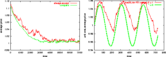
Figure 6: LEFT: Price adjustment. Bottom curve: when searching consumers compare prices. Top curve: when searching consumers accept prices no matter what they are. RIGHT: Prices tracking the cost of production.

As already mentioned above, it turns out that the price comparison by the consumers is not needed at all. We can replace the rule ``if price goes up, try to find a better price'' by ``if price goes up, go to a different shop no matter what the price there''. In both cases, we find the alternative shop via our neighbors, as we have done throughout this paper. The top curve in Fig. 6 shows the resulting price adjustment. Clearly, the price still moves towards the critical value of one, but it moves more slowly and the trajectory displays more fluctuations. This is what one would expect, and we think it is typical for the situation: If we reduce the amount of ``rationality'', we get slower convergence and larger fluctuations.

In terms of cluster size distribution, the price model is similar to the earlier spatial competition model with random injection. They would become the same if we separated bankruptcy and price changes.

In Fig. 6 (right) we also show that our model is able to track slowly varying costs of production. For this, we replace $C(Q)\; =\; Q$ by a sinus-function which oscillates around $Q$. The plot implies that prices lag behind the costs of production.

  
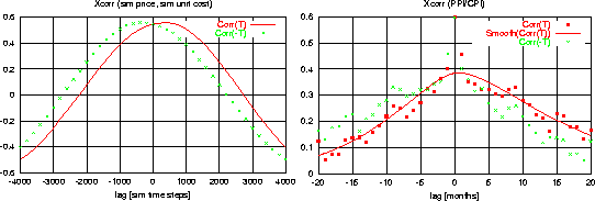
Figure: Crosscorrelation function between $R$_price and $R$_cost: $R$_X := X(t) / X(t-1); $XCorr(T)\; :=\; R$_P(t) R_C(t-T) . LEFT: Simulation. The crosses show the crosscorrelation values mirrored at the $T=0$ axis, in order to stress the asymmetry. RIGHT: U.S. Consumer price index for price and Producer price index for cost. Filled boxes are the crosscorrelation values; the smooth line is an interpolating spline for the filled boxes. The crosses show the crosscorrelation values mirrored at the $T=0$ axis.

This is also visible in the asymmetry of the cross correlation function between both series. In order to be able to compare with non-stationary real world series, we look instead at relative changes, $R$_x(t) = x(t) / x(t-1). The cross correlation function between price increases and cost increases then is $XCorr(\tau )\; =\; R$_P(t)   R_C(t-τ) , where $.$ averages over all $t$. In Fig. 7 (left) one can clearly see that prices are indeed lagging behind costs for our simulations. In order to stress the asymmetry, we also plot $XCorr(-\tau )$. In Fig. 7 (right) we show the same analysis for the Consumer Price Index vs. the Production Price Index (seasonally adjusted). Although the data is much more noisy, it is also clearly asymmetric.