Theoretical considerations

Spatial coarsening model (slope -2 in natural time)

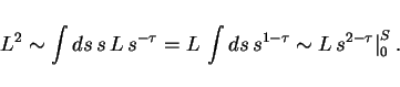
We are looking again at the ``basic model''. In cluster time this was: randomly pick one of the clusters, and give it to the neighbors. The following heuristic model gives insight:

1. We start with $N$ clusters of size 1.

2. We need $N/2$ time steps to delete $N/2$ of them and with that generate $N/2$ clusters of size 2.

3. In general, we need $N/2^k$ time steps to move from $N/2^{k-1}$ clusters of size $2^{k-1}$ to $N/2^k$ clusters of size $2^k$.

4. If we sum this over time, then in each logarithmic bin at $s=2^k$ the number of contributions is $N/2^k \times N/2^k$, i.e. $\sim s^{-2}$.

5. Since these are logarithmic bins, this corresponds to $\tilde n(s) \sim s^{-3} \hbox{ or } \tilde n(>\!s) \sim s^{-2} \ ,$ which was indeed the simulation result in cluster time.

6. In natural time, we need a constant amount of time to move from $k-1$ to $k$, and thus obtain via the same argument $n(s) \sim s^{-2} \hbox{ \ \ or \ \ } n(>\!s) \sim s^{-1} \ ,$ which was the simulation result in natural time.

Random injection in space (log-normal)

At the moment, we do not have a consistent explanation for the log-normal distribution in the spatial model. A candidate is the following: Initially, most injected clusters of size one are within the area of some larger and older cluster. Eventually, that surrounding cluster gets deleted, and all the clusters of size one spread in order to occupy the now empty space. During this phase of fast growth, the speed of growth is proportional to the perimeter, and thus to $\sqrt{s}$, where $s$ is the area. Therefore, $\sqrt{s}$ follows a biased multiplicative random walk, which means that $\log(\sqrt{s}) = \log(s)/2$ follows a biased additive random walk. In consequence, once that fast growth process stops, $\log(s)$ should be normally distributed, resulting in a log-normal distribution for $s$ itself. In order for this to work, one needs that this growth stops at approximately the same time for all involved clusters. This is apprixomately true because of the ``typical'' distance between injection sites which is inversely proportional to the injection rate. More work will be necessary to test or reject this hypothesis.

Injection on a line (slope -3/2)

If one looks at a snapshot of the 2D picture for ``injection on a line'' (Fig. 3), one recognizes that one can describe this as a structure of cracks which are all anchored at the injection line. There are $L$ such cracks (some of length zero); cracks merge with increasing distance from the injection line, but they do not branch.

According to Ref. [14], this leads naturally to a size exponent of $-3/2$, as found in the simulations. The argument is the following: The whole area, $L^2$, is covered by

$$\int ds \, s \, n(s) \ ,$$

where $n(s)$ is the number of clusters of size $s$ on a linear scale. We assume $n(s) \sim s^{-\tau}$, however the normalization is missing. If all clusters are anchored at a line of size $L$, then a doubling of the length of the line will result in twice as many clusters. In consequence, the normalization constant is $\propto L$, and thus $n(s) \sim L \, s^{-\tau}$. Now we balance the total area, $L^2$, with what we just learned about the covering clusters:

$$L^2 \sim \int ds \, s \, L \, s^{-\tau} = L \, \int ds \, s^{1-\tau} \sim L \, s^{2-\tau} \big\vert _0^S \ .$$

Assuming that $\tau < 2$, then the integral does not converge for $S \to \infty$, and we need to take into account how the cut-off $S$ scales with $L$. This depends on how the cracks move in space as a function of the distance from the injection line. If the cracks are roughly straight, then the size of the largest cluster is $\sim L^2$. If the cracks are random walks, then the size of the largest cluster is $\sim L^{3/2}$. In consequence:

• For ``straight'' lines: $L^2 \sim L \; (L^2)^{2-\tau}$ $\ \Rightarrow\$ $2 = 1 + 2 \, (2-\tau) %%= 1 + 4 - 2 \tau$ $\ \Rightarrow\$ $\tau = 3/2 \ .$

• For random walk: $2 = 1 + 3/2 \, (2-\tau) %% = 1 + 3 - 3 \tau/2 \ \ \Rightarrow \ \ \tau = 4/3 \ .$

Since our simulations result in $\tau \approx 3/2$, we conclude that our lines between clusters are not random walks. This is intuitively reasonable: When a cluster is killed, then the growth is biased towards the center of the deleted cluster, thus resulting in random walks which are all differently biased. This bias then leads to the ``straight line'' behavior. -- This implies that the $\sim s^{-3/2}$ steady state scaling law hinges on two ingredients (in a 2D system): (i) The injection comes from a 1D structure. (ii) The boundaries between clusters follow something that corresponds to straight lines. As we have seen, the biasing of a random walk is already enough to obtain this effect.

Injection without space (variable slope)

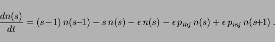
Without space, clusters do not grow via neighbors, but via random selection of one of their members. That is, we pick a cluster, remove it from the system, and then give its members to the other clusters one by one. The probability that the agent choses a cluster $i$ is proportional to that cluster's size $s_i$. If for the moment we assume that time advances with each member which is given back, we obtain the rate equation

$${d n(s) \over dt} = (s\!-\!1) \, n(s\!\!-\!\!1) - s \, n(s) ... ...t inj} \, n(s) + \epsilon \, p_{\it inj} \, n(s\!\!+\!\!1) \ .$$

The first and second term on the RHS represent cluster growth by addition of another member; the third term represents random deletion; the fourth and fifth term the decrease by one which happens if one of the members is converted to a start-up via injection. $\epsilon$ is the rate of cluster deletion; since we first give all members of a deleted cluster back to the population before we delete the next cluster, it is proportional to the inverse of the average cluster size and thus to the injection rate: $\epsilon \sim 1/\langle s \rangle \sim p_{\it inj}$. This is similar to an urn process with additional deletion.

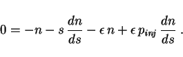
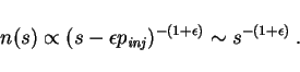
Via the typical approximations $s \, n(s) - (s-1) \, n(s-1) \approx {d \over ds} (s \, n(s))$ etc. we obtain, for the steady state, the differential equation

$$0 = - n - s \, {dn \over ds} - \epsilon \, n + \epsilon \, p_{\it inj} \, {dn \over ds} \ .$$

This leads to

$$n(s) \propto (s - \epsilon p_{\it inj})^{-(1+\epsilon)} \sim s^{-(1+\epsilon)} \ .$$

That is, the exponent depends on the injection rate, and in the limit of $p_{\it inj} \to 0$ it goes to $-1$. This is indeed the result from Sec. 3.4 (see Fig. 4).